Confidence Intervals and Point Estimates

More Statistics Topics
Confidence Intervals and Point Estimates

Confidence Intervals and Point Estimates

This chapter in Surviving Statatistics explains how to compute and use confidence intervals.

Instructional Videos

Surviving Statistics: Point Estimates & Confidence Intervals Business Statistics: Estimation & Confidence Levals

Confidence Intervals and Point Estimates

Point Estimate

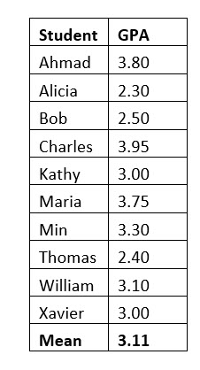
Based on what we learned about the sampling distribution of the sample means, if we want to estimate parameter values for a population, the best estimate of a population value is a statistic computed from a sample. If we wanted to estimate the mean GPA of the population of ten students, we could take a sample and compute the mean. That statistic, the sample mean, would be the best estimate of the population mean, assuming we did not have the values for the entire population.

However, while values derived from samples are the best estimates, we also know that a mean computed from a sample may not be exact due to sampling error. As we saw in the last chapter with the sampling distribution of the sample means, some sample means had a larger sampling error than other samples.

Confidence Interval

Because a statistic computed from a sample may not be exact, we use confidence intervals. A confidence interval is a range of values that we are confident contains the population parameter. We refer to our level of certainty, or confidence, as the confidence interval.

Confidence intervals are typically between 90% and 99%. So, using a 95% confidence level, you can be 95% confident that the true population parameter will fall within the confidence interval, the range of values less than and greater than the value we derived from the sample.

MARGIN OF ERROR – KNOWN POPULATION STANDARD DEVIATION

Confidence intervals use a margin of error. After computing the margin of error, we add and then subtract it from the sample mean to create the confidence interval (range). When we know the population standard deviation, we compute a margin of error based on a z score.

To understand this concept, let’s assume we want to accurately predict the population GPA for the ten-student class using a two-student sample. The sample we randomly selected was Ahmad and Kathy and the sample mean is 3.0

We want to be 95% confident in estimating the true population mean, so we choose a 95% confidence interval. We will create a range of values, centered around the sample mean of 3.0. Once we compute that range of values, we will have 95% confidence that the population mean lies within that range.

We know the population standard deviation is .5643. The formula for computing a margin of error from a sample mean is:

Notice that the margin of error formula is determined by the z score corresponding to the confidence level multiplied by the standard error of the mean.

The confidence interval equals:

We have the sample mean, 3.0, the sample size, 2, and the population standard deviation, .5643. Now, we must find the z score associated with a 95% confidence level. This z score will include 95% of the area under the normal curve.

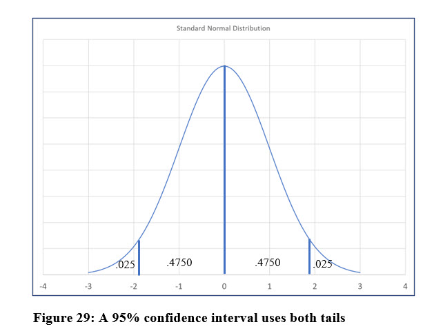
Because the confidence interval will be a range that is smaller and larger than the mean, we are looking for a two-tail z score. For a 95% confidence level, we are looking for a z score that represents 5% of the area under the curve. However, because we are adding and subtracting the margin of error to the sample mean, we will divide the 5% of the area not under the curve by two. Therefore, we are looking for a z score that represents 47.5% of the area between the population mean and the z score.

Using the normal distribution table, z scores, we locate the area of .4750 in the normal distribution table such as the one in Figure 28 on page 93, and find that area equates to the z score of 1.96.

Now we can compute the confidence interval based on the sample mean.

Margin of error = 1.96(.564/1.41) = .782

We add and subtract the margin of error to our sample mean and get a 95% confidence interval of 2.218 to 3.782.

We can be 95% confident that the true population mean (parameter) is between 2.218 and 3.782.

MARGIN OF ERROR – UNKNOWN POPULATION STANDARD DEVIATION

The previous formula for computing the margin of error assumes we know the standard deviation of the population, σ. If you are conducting new research on samples, it is unlikely you will have parameters such as the mean and standard deviation of the population. Although this may seem to create a problem because z scores and confidence intervals all require the population standard deviation. Statisticians have solved the problem by using another distribution.

The t distribution is similar to the z’s normal curve but is flatter and contains more information in the tails. The data in a t distribution is more dispersed from the mean than in a normal (z) distribution. We can compute t scores using the sample standard deviation, s, rather than the population standard deviation. Unlike z scores, t scores vary depending on the sample size. The t distribution accounts for the sample size in degrees of freedom.

The degrees of freedom for computing confidence intervals using a t score is n – 1.

Let’s see how this works with an example. Assume the GPAs from the ten-student course is now a sample of all statistic students in the college (the population). We want to create a 95% confidence interval for the means of the students in the college.

We will now consider the mean of these students as a sample mean, x̅.

The sample standard deviation, s, is .5948.

The formula to compute the margin of error is similar to the one used for z, except it uses the sample standard deviation and a critical t value, not z.

Since we have the standard deviation and the sample size, the next step is to look up the t score in the t distribution table.

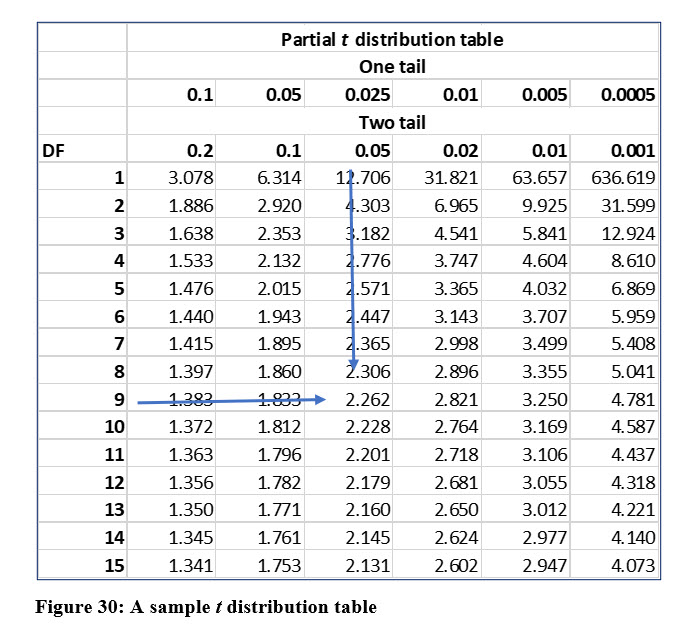
As previously mentioned, the t distribution uses degrees for freedom, which in this case will be n – 1, or 9 for this sample of 10 students.

A confidence interval includes values both greater than and less than the mean, so the t score will also be a two-tailed, just like the z score was.

Some t distribution tables display columns for both one and two tail tests. This may actually be more confusing than helpful. Either way, the column we want is the .05 two tail or .025 one tail (2.5% in each tail). After locating the degrees of freedom row and the confidence level column, you can then locate the t score, which in this case is 2.262 as you can see in Figure 30.

You should notice that the t score for the 95% confidence, 2.262 is larger than the z score for the same level, which was 1.96. T scores are larger because the curve is flatter than a z distribution, which, again, means there is more dispersion from the mean.

The margin of error for a 95% confidence interval using the t distribution is: 2.262((.5643/1.414) = .903

The 95% confidence interval is: (2.207, 4.013). We can be 95% confident that the population mean falls within this range.

Z OR T?

If you have the population standard deviation, use the z distribution. If not, use the t distribution.

CONFIDENCE INTERVALS FOR PROPORTIONS

Proportions are fractions, ratios, or percentages of the whole that possess a specific trait, attribute, or interest. Examples could include the percentage of statistics students who failed the course compared to all statistic students we sampled. Or the proportion of products coming off the assembly line which failed final inspection compared to all products we sampled that day.

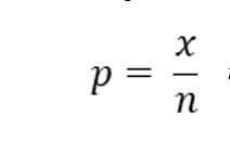
Proportions rely on the nominal measurement scale and there are only two possible outcomes. Often these are attributes that can be answered with a yes or no, or pass or fail. The formula to compute the sample proportion is:

x is the number with the attribute (answered yes, passed, etc.…) n is the sample size

For our example, we will assume we sampled 100 moviegoers and asked each if they liked the last movie they watched. Forty of our sampled moviegoers answered “yes”. The sample proportion is 40/100 or .4.

We want to compute the 95% confidence interval for this sample proportion.

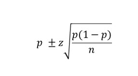
The formula to compute a confidence interval for a sample proportion is:

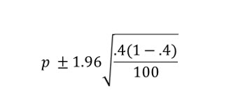
Notice that proportions use the z statistic, even though we do not have the population standard deviation. We know from past examples, that the z score for a 95% confidence level, two-tail, is 1.96. So, we compute the margin of error as:

The margin of error is .096, so the confidence interval becomes: .304 to .496 .

This means we can state, with 95% confidence that the proportion of movie goers who liked the last move they saw falls between .304 and .496.

CHOOSING A SAMPLE SIZE

As we have seen with many computations already, the sample size is a very important factor. We also saw with the central limit theorem that the larger the sample size, the more the sampling distribution of the sample means approaches a normal distribution curve.

So what is the optimal sample size? Computing the correct sample size depends on three variables: 1. The maximum acceptable margin of error. 2. The desired level of confidence. 3. The dispersion of the variable being studied in the population (standard deviation).

Sample Size for Population Mean

When you are attempting to determine the proper sample size, you will use one formula when you are measuring means and another for preparations. We will begin with the formula for choosing a sample size for estimating population mean values.

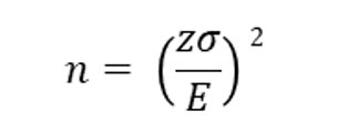
The formula for computing a sample size is:

In this formula, E is allowable margin of error. We’ll discuss this in the example.

As an example, assume you want to estimate the GPA of all the students at a particular college taking statistics. You do not want to survey the entire population, so you decide to survey a sample. Assuming you want a 95% confidence level, and are only willing to accept a margin of error of 0.1, or 10%, how many students do you need to survey?

You should have noticed that we are missing one required variable to compute the sample size, the population standard deviation. While we could probably get this information from the college’s administration, we will assume they have very bad records, or are unwilling to assist in our research, so we cannot procure that value.

As we have already discussed, when you are doing your own research, you will often be unable to procure values relating to the population, such as the standard deviation. So, does that mean we cannot compute a sample size? Fortunately, there are ways we can estimate this unknown value.

Ways to estimate the population standard deviation include: 1. Use data from previous studies, or conduct a pilot study 2. Estimate the standard deviation from the population range. If you know the possible range, you can then divide the range by 4 or 6, to estimate the population standard deviation. Why either 4 or 6? If the population range is correct, it will include all possible values. Recall that the empirical rule tells us that 99.7% of the values fall within +/- three standard deviations of the mean, which totals six. The empirical rule also tells us that 94.7% of the values fall within +/- two standard deviations of the mean, which totals four. For our example, we will divide the rage by six. For our example, GPA’s can range from 0 to 4. The range is four. Our estimated population standard deviation is 4/6 = .667

Now we can compute the correct sample size:

The z score of 1.96 represents the 95% confidence interval, 2.5% in each tail.

We have computed a required sample size of 171. This is much larger than the ten-student sample size we have been using. A sample size of 10 would be the appropriate size if we allowed a margin of error of .4.

Sample Size for Proportions

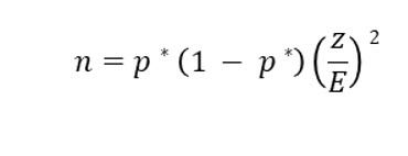
As we have already discussed, we do not use standard deviation when we compute statistics for proportions. The sample size for proportions uses the population proportion and the margin of error.

n this formula, p* is the population proportion. If you do not know this, you can estimate it. We can estimate the population proportion by: 1. Conducting a pilot study 2. Using previous studies 3. Using your “best guess” 4. Using 0.5 as an estimate

We will continue to work in proportions in upcoming chapters.