Sampling and Sampling Distributions
This chapter in Surviving Statatistics explains different sampling methods and how sample data can be representative of population data.
Note: This chapter is excerpted from Luther Maddy’s Surviving Statistics textbook (C) 2024 which is available in printed or eBook format from Amazon.com
Instructional Videos
Surviving Statistics: Sampling Distribution of the Sample Mean
Business Statistics: Sampling Methods
Surviving Statistics - File Downloads
Student GPA Sampling Distribution
Sampling and Sampling Distributions
We have already discussed the differences between a sample and a population and statistics and parameters. We have discussed several reasons why we use samples instead of populations. In this chapter we will discuss how to properly select a sample. We will also show why we can trust samples to be representative of a population.
Sampling methods
Some of the sampling methods you should be aware of include:
SIMPLE RANDOM SAMPLING
To ensure the sample represents the population, every object or person in the population should have an equal chance of being selected. With simple random sampling, selection of any one object to be included in the sample occurs at random. No one item or person, or group of persons or items, is selected beforehand or targeted to be sampled. Practical examples of this include drawing a name out of a hat. If all names have an equal chance of being selected, then the name drawn was completely random.
If you decide to use this method, you can use a table of random numbers which are usually included in textbooks or available online. You can also use Excel to generate random numbers as well.
SYSTEMATIC RANDOM SAMPLING
With systematic random sampling, you take a list of the population you want to sample and then take every kth item. For example, in a list of 100 employees, you may decide to survey every 5th employee.
Sampling error
In most cases, properly collected and sized samples are representative of the population. We will understand why we can trust this statement when we discuss sampling distributions shortly. However, because the sample is not a perfect representation of the population, there will be a difference between the statistics computed from the sample and the parameters computed from the entire population.
We refer to the difference between the sample statistic and the population parameter as the sampling error.
Sampling Distribution of the Sample Mean
You should recall that a probability distribution is a listing of all possible outcomes and the probability of each outcome. Similarly, a sampling distribution of the sample mean is a listing of all possible sample means you can generate from a particular sample size, n.
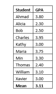
To illustrate a sampling distribution of the sample mean, assume a certain statistics class has 10 students. You want to know how your own GPA compares with the average GPA of the class as a whole. So, you have decided to select two students at random and compute the mean GPA of those two students. Each student in the class and their GPA is shown below.
Is the mean of the two-student sample an accurate representation of the population (class) mean? Let’s see.
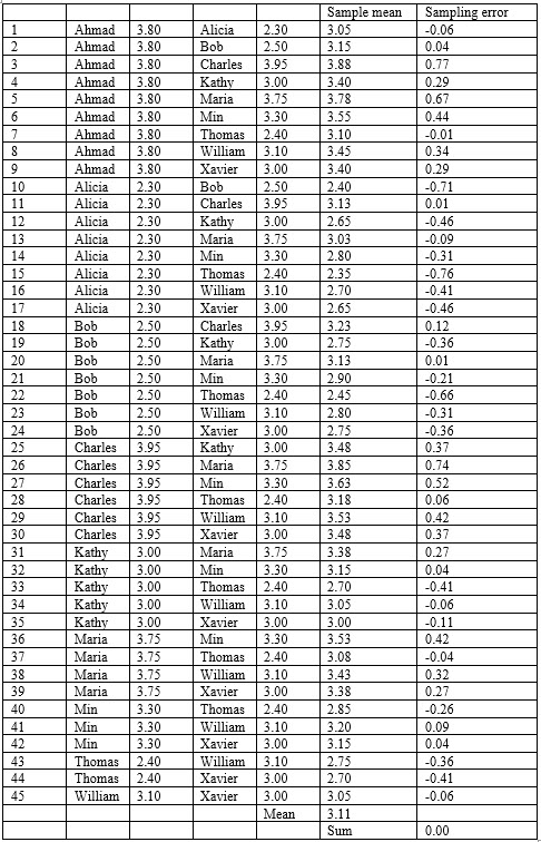
With a sample size, n, of 2 and a population, N, of 10, there are 45 possible samples of two student each. We use the combination formula to tell us home many possible combinations were possible.
The sampling distribution of the sample mean lists all possible samples of two and the computed mean of each possible sample.
The following table shows every possible two-student combination, 45 in all, and the mean of that sample. The difference between the sample mean and the population mean is the sampling error. Notice that the mean of the sample means is exactly equal to the population mean.
Also note the sum the sampling error in the distribution is zero. The important concept here is that samples can accurately represent the population.
The Central Limit Theorem
The central limit theorem states that a sampling distribution of the sample means can be approximated by a normal distribution. The larger the sample size, the closer to a normal distribution the sampling distribution of the sample mean becomes.
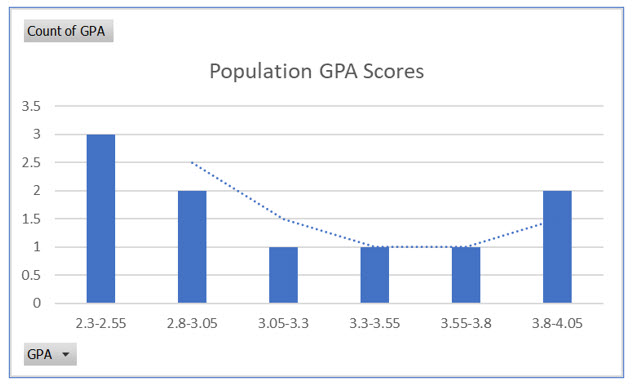
Even with a sample size of two, as in the class GPA example, you can see the central limit theorem expressed. The first illustration is the frequency distribution to the population GPA scores. For ease of interpretation, the scores are grouped with a width of .2.
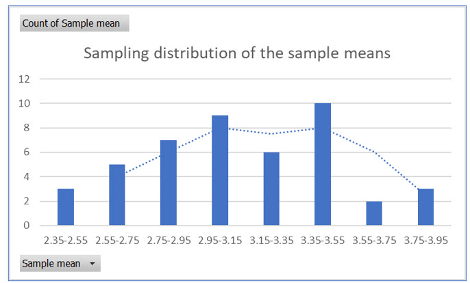
The second illustration is a frequency distribution of the sampling distribution of the sample means for a sample size of two. You should notice that even with an extremely small sample size, the distribution begins to approximate a normal distribution.
So, what is the big deal about the central limit theorem? It lets us assume that our sample data can be represented with a normal distribution. This allows us to use sample means and compute z scores. This, in turn, lets us compute probabilities or areas under the curve with the z scores computed from our sample means. As you progress through statistics, you will often see the words “assume the data is normally distributed” in practice problems and examples. We can make this assumption based on the central limit theorem.
Using a Sample Mean to Compute a Z score
Up to this point we have computed z scores using one value, x. Since statistics is concerned with samples, we will also want to compute z scores based on sample means.
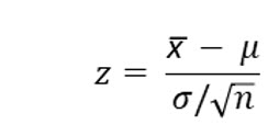
Here is the formula we use to compute a z score from a sample mean.
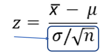
Notice that the sample size is an integral part of this equation.
Here is an example of this equation in action. In the ten-student class discussed previously, we computed the population mean of the GPA to be 3.11. While we did not compute it, the standard deviation of this population is .5643.
Assume we wanted to find two representative students and their GPAs from the course. We randomly select a sample of two students, Alicia and Bob. The mean of this sample, x̅, is 2.40.
Are these two students a good representation of the class as a whole?
Or, since the sample mean is less than the population mean, what is the probability of finding a sample with this GPA or lower?
Using the z score formula we solve for z as: (2.40 – 3.11) / (.5643/1.414) = -1.78
1.414 is the square root of the sample size, 2.
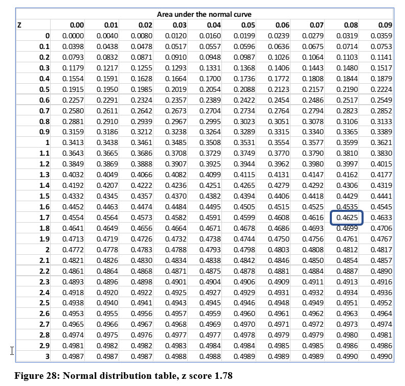
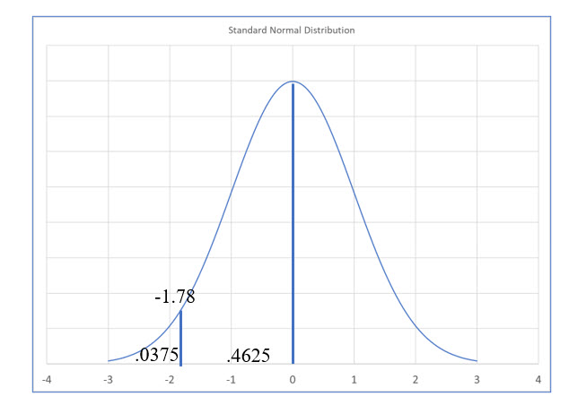
The z score is negative because the sample mean is less than the population mean. Now, we find the probability (area), associated with a z score of 1.78. Using the normal distribution table which we have placed on the following page in Figure 28, we find the area to be .4625.
How do we interpret this?
The chances of finding a sample mean lower than this is 3.75%. The chances of finding a sample mean higher than 2.4 is 96.25%. The sample we took is not the best representation of the typical students in the course. Here we see an example of sampling error. We also see why larger sample sizes are important, as well as why we should conduct multiple samples when possible.
Even though the two students we selected at random do not perfectly represent the typical students, if we sampled enough students, we would arrive at a mean GPA very close to the population mean GPA.
Standard Error of the Mean
The denominator of the formula you just used to compute a z score based on a sample mean is called the standard error of the mean, or more accurately, the standard deviation of the sampling distribution of the sample mean.
You will use the standard error of the mean as a stand-alone computation. You will also use other upcoming computations, such as confidence intervals, which we will discuss in the next chapter.

