Continuous Probability Distributions
This chapter in Surviving Statatistics explains measures of continuous probability distributions including uniform and normal distributions. This chapter also introduces working with Z scores.
Note: This chapter is excerpted from Luther Maddy’s Surviving Statistics textbook (C) 2024 which is available in printed or eBook format from Amazon.com
Instructional Videos
Surviving Statistics: Uniform & Normal Proability Distributions
LaBron James -50 point game. What are the odds?
Business Statistics: Continuous Probability Distributions
Chapter 7 - File Downloads
Z Score Calculator- One Mean (Excel file)
Z Score Calculator- Sample Mean (Excel file)
Continuous Probability Distributions
Uniform Distributions
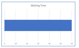
In a uniform probability distribution, the probability of any outcome is equal to that of any other. To illustrate this, assume you have arrived at a bus stop. The bus is not there and so you must wait for it to return. The schedule of times is missing, but you know a bus arrives at this stop every 60 minutes. You do not know when the bus was last here, so your waiting time can be from 0 to 60 minutes. And, the probability of your waiting time, with your lack of knowledge, is uniform for any of the times in that range.
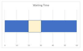
Uniform probability distributions are represented as a rectangle with the minimum and maximum values.
Since this is a uniform distribution, the probability of any point in the rectangle is the same as any other. The probability of you waiting 10 minutes is equal to your waiting 50 minutes.
As you are waiting for the bus, you will invariably want to know the probabilities of different waiting time scenarios.
For example:
1. What is the mean (expected) wait time?
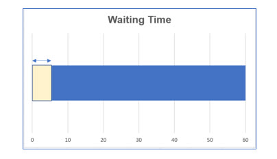
2. What is the probability you will have to wait 5 minutes or less?
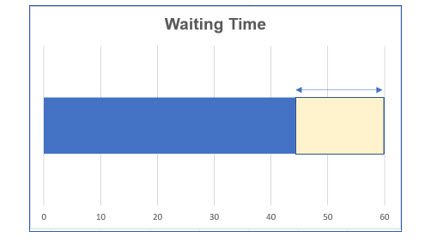
3. What is the probability you will have to wait longer than 45 minutes?
Here are the computations to answer your questions.
The mean of a uniform distribution:
To answer the other questions, take the following steps:
1. Compute the probability of any one point in the distribution. The probability is computed as:
2. Determine the number of units you are determining the probability for.
5 minutes or less: 0 + 5 = 5.
3. Multiply the number of units by the probability of each unit, minutes in this case.
(5)(1/60) = 5/60 = .08333
What is the probability you will have to wait longer than 45 minutes?
a. 60 – 45 = 15
b. (15)(1/60) = 15/60 = .25
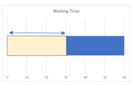
What is the probability you will have to wait 30 minutes or less?
a. 0 + 30 = 30
b. (30)(1/60) = 30/60 = .5
What is the probability you will have to wait between 20 and 30 minutes?
a. 30 – 20 = 10
b. (10)(1/60) = 10/60 = .1667
Normal Probability Distributions
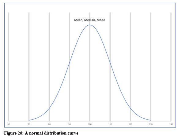
A normal curve is represented by a bell-shaped curve. In a perfectly normal distribution, the mean, mode, and median are all the same. The mean is represented by the top of the curve and most of the data points are distributed closely around the mean.
The standard deviation is also an important value in a normal probability distribution. The empirical rule, which we previously discussed in Chapter 3, uses the standard deviation to determine the percentage of data points that fall within 1, 2, or 3 standard deviations of the mean.
Just to refresh your memory, the empirical rule states that approximately 68% of the data points fall within + or – 1 standard deviation of the mean. Using the illustration below, with the empirical rule in mind, if we pick a data point in this distribution at random, there is a 68% probability that the value will fall between 90 and 110.
STANDARD NORMAL DISTRIBUTION (Z SCORES)
The standard normal distribution and z scores makes it easier to compute probabilities and areas under the curve. Instead of working with innumerable values for means and standard deviation, the computed z score reports how many standard deviations a value varies from the mean. Knowing the z score for a value, we can then compute the area under the curve, or probability.
This will make more sense as we step through an example.
The formula for computing a z score is:
Using the previous illustration, the mean for this distribution is 100 and the standard deviation is 10. Please note that we used σ to designate the standard deviation, which indicates this is a population value, not one derived from a sample.
Assume we want to know the probability of choosing a data point higher than 110 at random. With this illustration, it is easy to determine that the value of 110 is 1 standard deviation higher than the mean. With “real world” examples, it isn’t always that easy so let’s step through computing a score with those values and then build on that example.
Recall that the z score tells us how many standard deviations the value varies from the mean, which in this case is 1.
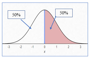
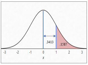
The illustration below shows the area of the normal curve we are trying to quantify, the area (probability) of having a z score > 1, which represents a value of 110.
The shaded area is all the area to the right of the z score because we are concerned with a score of 110 or higher, which is a z score of 1.
To determine the probability of finding a score of 110 or greater in this distribution, we need to know how much of the curve is taken up with the shaded area.
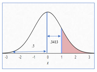
o determine the area within the curve for a z score, the first important concept is to realize that the curve is essentially divided by 2. The mean marks the position where half of the curve represents a value less than the mean and the other half represents values greater than the mean.
It should be obvious that a z score of 1.0 will represent less than 50% of the curve’s area.
Computing the probability, area of the curve, for a z score manually is somewhat complex and time consuming. Using software like Excel makes this easier.
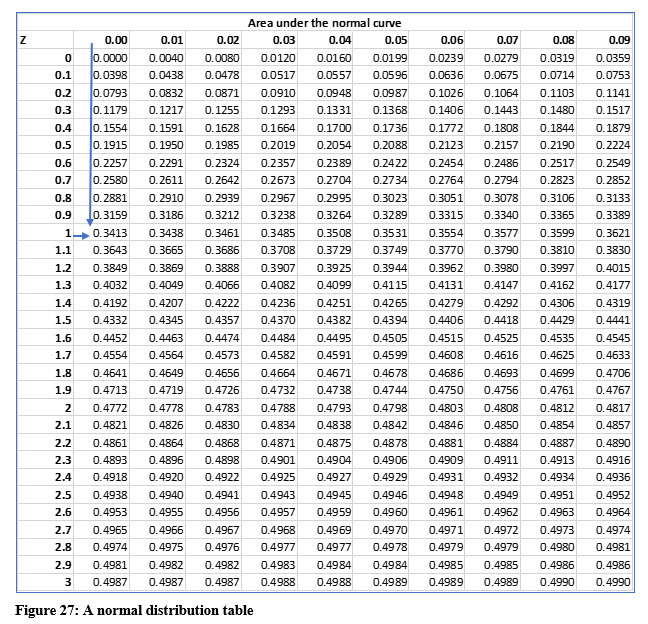
Most textbooks include a table similar to Figure 27. You can easily use this table to find probabilities for z scores. We will use this table as we continue to follow the example.
Using the table, the area under the curve associated with a z score of 1.0 is .3413.
After finding this value, you may be tempted to answer the question, “What is the probability of finding a score above 110?” with 34%. However, the answer is not quite that simple.
The area you located, .3413, represents the area of the curve from the mean to that z score.
Knowing that the each half of the curve is .5, we can now use the value we found in the table to compute the area of the curve represented by the shading.
= .5 - .3413 = .1587
So, the probability of finding a data point with a value higher than 110 is 15.87%.
So, let’s approach this another way.
What is the probability of finding a value data point with a value lower than 110?
We still use the area we located in the table, .3413, but that is still not the complete answer. Because we are looking for any value lower than 110, the value could also be lower than the mean. To account for this, we must include the area from the mean to the z score of 1, and the entire half of the curve to the left of the mean.
So, the probability of finding a data point with a score lower than 110 is:
.5 + .3413 = .8413
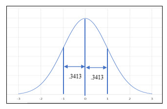
Now, what if we wanted to know the probability of finding a data point with a value between 90 and 110?
The z scores are: (110 – 100) / 10 and (90 – 100) / 10
= 1 and -1
While some normal curve probability tables will display areas for negative z scores, some, like the example on the previous page, do not. If the table you are using does not have values specifically for negative z scores, you can use the absolute value of the z score 1, for -1, and use the value associated for that value, but continuing to realize the score represent a position in the curve to the left of (less than) the mean.
The probability of finding a data point with a value between 90 and 110 is:
.3413 + .3413 = .6826
Solving for x
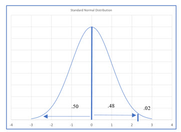
Sometimes you will be given an area or probability and then be asked to find the value that relates to that probability. For example, Oliver’s Outboards makes and sells outboard motors for boats. After several years in business, Oliver knows that his outboards fail, on average, after 500 hours of use with a standard deviation of 22 hours. (Oliver is a data geek.) Oliver wants to offer his customers a warranty but is willing to have only 2% of his motors fail during the warranty period. What warranty, in running hours, should Oliver offer on his outboards?
We are solving for x in this case, the number of hours. The steps in doing this are:
1. Find the z score associated with the top 2%.
Using the table, we locate a z score for the area of .48.
The z score is between 2.05 and 2.06. Using the table, we can approximate with 2.055. Using Excel or the formula, we compute an actual value of 2.054. We will use 2.055 in our computations.
2. After finding, z, use algebra with the z score formula to solve for x.
That formula becomes:
Add if the value is higher than the mean and subtract if less. Since Oliver wants 98% to last longer than the warranty period, this value will be less than the mean.
x = 500 - 2.054(22) = 454.812
So, Oliver should offer a warranty close to 454.812 hours to ensure that only 2% or less of his motors fail during the warranty period.
Try it in Excel:
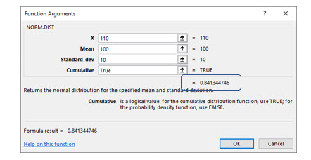
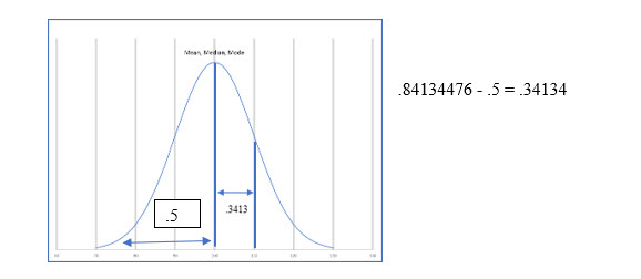
Excel’s Norm.Dist() function will compute the area under the curve for a given value. For this to work properly, you will turn on the Cumulative argument. However, this causes Excel to add .5 to the area because it includes both halves of the curve. The images show Excel’s solution.
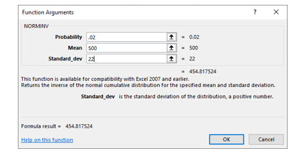
In situations where you need to solve for the x value, you can use Excel’s NormInv() function.
