Discrete Probability Distributions

More Statistics Topics
Discrete Probability Distributions

Discrete Probability Distributions

This chapter in Surviving Statatistics explores Discrete proability distributions including Binomial and Poisson distributions.

Instructional Videos

Surviving Statistics: Discrete Proability Distributions Business Statistics: Discrete Probability Distributions

Chapter 6 - File Downloads

Dice Probability Distribution

Binomial Distribution - Fish Shipping

Coffee Customer Arrival - Poisson Distribution

Discrete Probability Distributions

Probability Distributions

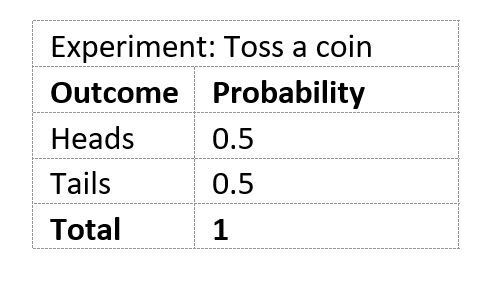
A probability distribution lists all possible outcomes from an experiment. It also lists the probability of each possible outcome. To be a true probability distribution the sum of all the probabilities listed must equal 1 or 100%.

Before we dive deeper into probability distributions, here a few terms we need to discuss.

RANDOM VARIABLES

A random variable is a numeric value that results by chance from an experiment. The result of rolling a die or flipping a coin is a random variable. The weight of a two-year-old, selected by chance, is also a random variable.

Discrete Random Variable

We previously defined a discrete variable as the result of counts. A discrete random variable is the result of an experiment that is selected by chance and the resulting value can be counted. An example of a discrete random variable could be the number of cars driving through an intersection in a ten-minute period.

Continuous Random Variable

A continuous variable can assume any value and often results from measurements. For example, the weight of a two-year old selected at random would be a continuous random variable. We will discuss probability distributions for continuous random variables in an upcoming chapter.

DISCRETE PROBABILITY DISTRIBUTIONS

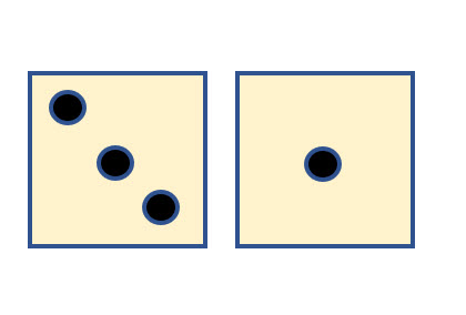
A discrete random variable often assumes a value that can be counted. This is the case with rolling dice. To understand this concept of a discrete probability distribution, let’s use the experiment of tossing 2 six-sided dice. The results are counted.

You cannot roll two dice and get 2.3 or 2.4. You will get only whole numbers, which is often the case of discrete variables. Two dice with six outcomes results in 36 possible outcomes, (6)(6) using the multiplication formula.

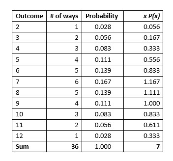
1. The first step in creating a probability distribution is to list all the possible outcomes and the number of ways or expected frequency of each outcome as shown.

2. The next step is to compute the probability of achieving each outcome. You do this by dividing the frequency of the outcome by the total number of outcomes, 2/36 for example. If all the probabilities sum to 1, you have accounted for all outcomes and have a probability distribution.

Expected Value or Mean of a Discrete Probability Distribution

As you can see from the probability distribution, some outcomes are more likely to result from throwing two dice than others. The outcome with the highest probability is 7. If we toss two dice, what value do we expect, on average, to see?

To compute the mean or expected value of a discrete probability distribution, multiply each outcome by its probability and sum the results.

The expected value, or mean, of rolling two dice is 7.

Variance of a Discrete Probability Distribution

The variance is a measure of dispersion as you learned previously. However, the formula you used in the previous chapter does not apply when dealing with a discrete probability distribution. The formula for computing the variance is:

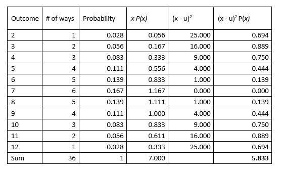
The steps in computing this are: 1. Subtract the mean from the value of each outcome and square the difference. 2. Multiply the squared differences by the probability of that outcome. 3. Sum the squared differences multiplied by the probability.

The variance of this discrete probability distribution is 5.833.

The standard deviation is the square root of the variance, in this case: 2.415.

Try it in Excel:

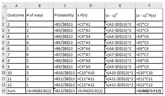
Excel has no built-in functions to compute the mean and variance of a discrete probability distribution. However, it is a great calculator if you create the formulas manually. The image below shows one way to approach these calculations. The image displays the formulas used in those computations.

BINOMIAL PROBABILITY DISTRIBUTIONS

Binomial probability distributions are another type of discrete (countable) probability distribution. However, in a binomial distribution there are only two possible outcomes. A binomial distribution output might be pass or fail, yes or no, late or not late, purchase or not purchase, or even live or die. With a binomial probability distribution, the probability of any one success or failure is the same, no matter how many trials are done.

For example, Juan is a tropical fish breeder. He ships his fish from Florida to anywhere in the United States. From past experience, Joe has discovered that each fish he ships has a 95% chance of making it through the shipping process and arriving alive. Juan wants happy customers, so he throws in an extra fish or two with every order. This way he ensures the customer will receive at least the number of fish he or she ordered alive. However, Juan still needs to make a profit, so he wants to know exactly how many extra fish to ship.

So, if a customer orders 6 fish, what is the probability all fish will arrive alive and that none of the fish, 0, will be dead on arrival (DOA)?

What is the probability that 1 of the 6 fish shipped will die in the process?

What are the probabilities that 2, 3, 4, 5, or all 6 will die in transit?

To solve this dilemma, Juan resorts to something he learned about in his statistics course, the binomial probability formula.

The Binomial probability formula is:

Where: px = the probability of x number of successes nCx = Combination, where n is the number of trials p = the probability of a success on each trial

For Juan’s example, we will consider a success (outcome we are concerned about) as arriving deceased. The probability of any one fish not making it is 0.05. So, what is the probability that none, 0, of the 6 fish will die in shipment?

Let’s step through this computation. We are calculating the probability of 0 fish dying during shipment, P(x) with x = 0 We are shipping 6 fish, so n = 6. The probability of any one fish dying during shipment, p, is 0.05. Any value to the power of 0 equals 1, so p0 = 1. The combination of n = 6 and x = 0 also equals 1.

The probability that all the fish will live, none of the fish will die in shipment is 74%.

What is the probability exactly 1 fish will die in shipment?

The probability that exactly 1 fish in 6 will not survive shipment is 23.21%.

What is the probability that the shipment of 6 fish will arrive with 2 DOA fish? That computes to .0305.

Binomial Probability Distribution Tables

Binomial probability computations can be somewhat time consuming. Because of that, statistics textbooks often include tables like the one on the one shown in Figure 24. The binomial probability distribution tables are set up so that if you know the number of trials, six with Juan’s fish example, and the probability of success, 0.05 in the example, you can then use the table to find the probability.

Examine the table in Figure 24. To solve the first scenario, 0 fish die in shipment, we first find the table a trial size, n of 6. This is the correct table. Then, locate the 0.05 probability column, the probability of any one success that Juan already knew. According to the table, the probability of 0 fish dying in shipment is 0.735, just what we computed.

When you use a Binomial table, first note that you are using the correct table based on the number of trials. Then, find the value where the number of successes and the probability intersect to find the probability of that number of successes.

To finish up with Juan, with a shipment of six fish, he will throw in two extra fish. By doing this, he is nearly 95% sure that his customers will receive all the fish they ordered, and possibly even an extra one or two.

Mean - Binomial Distribution

Computing the mean of a binomial distribution is not difficult. It is simply the number of trials, 6 for Juan’s fish, multiplied by the probability of success for each trial, 0.05 in the example.

So, with Juan and his fish, the mean of fish expected to die in shipment is (6)(.05) = .3

Variance - Binomial Distribution

Like the mean, computing the variance of a binomial distribution is also easy. The formula to do so is:

Try it in Excel:

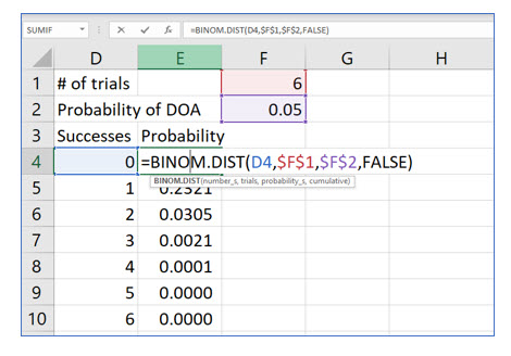
Excel’s Binom.Dist() function will compute probabilities for x number of successes. You will need to provide the number of trials and the probability of success. As you see in the illustration, you can also use this function to create your own Binomial Probability Distribution tables. The “FALSE” at the end of the function informs Excel that you do not want to create a cumulative probability table, but instead want it to display the probability for each number of successes.

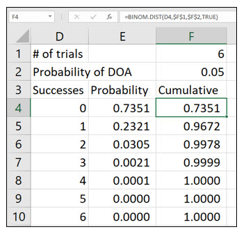
The cumulative probability adds the probabilities for each number of successes. So, as you can see in this illustration, there is a 96.72% probability of having <=1 successes, which for our example, is fish dying in shipment.

POISSON PROBABILITY DISTRIBUTIONS

The Poisson distribution is considered a discrete distribution because it also relies on counting. The Poisson distribution also needs a specific interval of time or space. For example, the Poisson distribution is helpful to determine how many customers will come into a store in a specific period of time. The Poisson distribution could also be used to predict the number of potholes on a given stretch of freeway, or the number of bears in a square mile of forest wilderness.

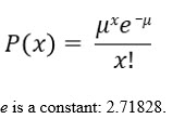
The binomial distribution required that we have probability of success to determine the probability of exactly x successes. With the Poisson distribution, the probability is determined with the mean number of occurrences. Once the mean is determined, the probability of x successes can be determined using the Poisson distribution formula, which is:

To see how the Poisson distribution works, assume Kathy is considering hiring another barista for her drive-through coffee stand. It takes approximately five minutes to process an order from start to finish which means her current barista can adequately handle three customers every fifteen minutes. Kathy knows that her customers become impatient if they must wait too long. Yet, she wants to maximize her profits and does not want to hire another barista if unnecessary.

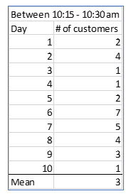
One of Kathy’s busiest times is between 10:15 and 10:30 in the morning. To see if she needs to hire another barista, Kathy records the number of customers arriving each day during this time period for ten days.

Using this information, Kathy sees that on average, three customers arrive during this fifteen-minute period. At first glance, it seems her current staffing of one barista is adequate. But, to be sure, Kathy wants to know the probability of four customers arriving during that time, which means one customer may end up choosing to purchase coffee elsewhere.

Using a mean of three, Kathy can now use the Poisson distribution to compute the probability of four customers arriving from 10:15 – 10:30.

Kathy learns there is nearly a 17% chance of having exactly 4 customers show during this time period.

However, Kathy wants to know more. What is the probably of having 5 or 6 or 7 or even more customers show up during this time period?

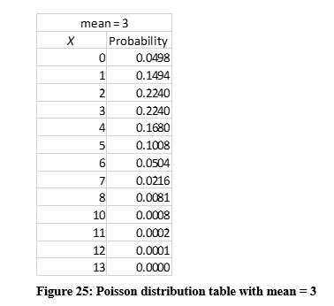
Fortunately, like the Binomial distribution, most textbooks have Poisson distribution tables that allow you to easily look up a specific or cumulative probability. Using a table, such as the one illustrated in Figure 25, Kathy can get the vital information she needs.

The probability of more than 3 customers arriving during this time period is easily calculated by (1 – the probability of 0, 1, 2, or 3). The cumulative probability of 0, 1, 2, or 3 customers is .6472. So, the probability of having more than 3 customers is 1 - .6472, or .3538.

Kathy decides the probability of losing customers is too great, more than 35%, so she decided to hire another barista in the morning. She will continue to track the number of customers to see if the mean number of customers she originally computed is accurate.

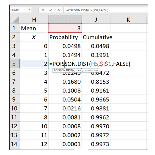
Try it in Excel:

Excel’s Poisson.Dist() function allows you to compute an individual probability or create a Poisson distribution table. By changing the cumulative argument from False to True, you can also create a cumulative probability distribution.