Chapter 3: Descriptive statistics – Numerical Methods

This chapter in Surviving Statatistics explains measures of central tendency and dispersion. It will cover mean, mode, median, variance, standard deviation and more.

Note: This chapter is excerpted from Luther Maddy’s Surviving Statistics textbook (C) 2024 which is available in printed or eBook format from Amazon.com

Instructional Videos

Video - Statistical methods 3a: Mean, mode, and median

Video: Statistical methods 3b: Range, variance, standard deviation

Video: Business Statistics: measures of central tendency

Video: Business Statistics: measures of dispersion

Surviving Statistics - File Downloads

Student Quiz Scores

Descriptive statistics – Numerical Methods

Measures of Central Tendency

While frequency distributions tell us how many observations are in a category or within a specific range, there are additional methods we can use to describe the variables in our dataset. Among these are measures of central tendency. These measurements try to answer the question, “What does the average observation look like?” To answer this question, we will use the arithmetic mean, mode, and median.

The Mean

The mean is the “average” computation you learned to compute in your early school years. In statistics, we use “mean” because the word “average”, to the “average” person (mathematicians excluded), can mean any one of the three computations we just mentioned.

In statistics, the mean is the mathematical center point of the dataset. You compute the mean by adding every value in the dataset and then dividing the sum by the number of items you added.

Population Mean - µ

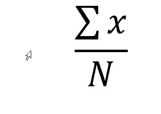
The population refers to all members of the group. (I know we already covered that, but repetition is essential in education.) The total number in the population is represented with a capital N. To compute the mean of the population, sum all the values of the variable of interest (x), and divide that by the population size, N. The population mean is represented by the Greek letter mu (µ).

Sample Mean – x̅

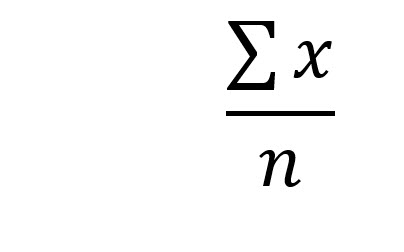
The number in the sample, the sample size, is represented with a lowercase n. We compute the sample mean the same as the population mean: sum all the values of the variable from the sample and divide the sum by the sample size, n. The sample mean is represented by the symbol x̅.

As we progress through this subject, we will find that we need to know if we are looking at a sample mean, or a population mean. That is why we represent them differently, µ for population mean and x̅ for sample mean. With some upcoming computations, we will compute the population and sample values differently.

Try it in Excel:

In this example, the 10 values for x are summed and then the sum is divided by n. (We are assuming this is a sample.)

In Excel, you can save a step by using the Average() function as shown. Note that Excel uses the term average, instead of mean, for this function.

It’s Greek to me

To this point, we have not used too many Greek symbols, but we have introduced some symbols and letters used in statistics.

You probably wondered why we needed separate formulas for the population and sample means when they were the same formula. As you progress in statistics it will be very important to differentiate whether the values you are using in formulas are from a sample or a population. Some of the computations in this chapter and beyond are different if you are working with a population rather than a sample.

So, let’s summarize the symbols we have used so far:

PARAMETERS VS. STATISTICS

Numerical characteristics of a population, such as the mean (µ), are called parameters.

Numerical characteristics of a sample, such as the mean (x̅), are called statistics.

Do you remember the definitions of statistics from the first chapter? Now we can complete the second definition:

Statistics are organized, analyzed, presented, or interpreted quantitative data (numbers) based on sample data.

So then,

Parameters are organized, analyzed, presented, or interpreted quantitative data (numbers) based on population data.

The mean and outliers:

Because the mean includes every value in its computation, it is susceptible to outliers. To see how this works, assume that your statistics teacher has created a new quiz. There are seven students in your class, and they scored as follows:

After giving the quiz, your teacher asks for feedback on the difficulty of the quiz. Student #1, (probably you), has no problem with the quiz. It may have even been too easy. The other six students complain loudly. The quiz was far too difficult because none of them received a grade that will help them earn at least a “C” in the course, which is considered the lowest passing grade.

Your statistics teacher gets defensive. “I did some statistical analysis, and the mean quiz score was 72. That’s exactly what the mean grade should be, a ‘C’.”

He is the teacher and you are the student, and if you are not student #1, you assume he knows what he is talking about. Still, something doesn’t seem quite right with his analysis.

You have just experienced a limitation of the mean, which is commonly called the average. Because the mean includes every value in the dataset, it can be skewed higher or lower by a value or two that does not fit the rest of the values. In this example, student #1’s score is not truly indicative of how the “average” student scored and neither is the computed mean of 72.

MEDIAN – LOCATIONAL CENTER POINT

Because the mean can be skewed by outliers, sometimes the median becomes a more accurate measure of the central tendency. The median is the value that lies in the middle location of the observations. There are an equal number of observations below and above the median.

To find the median:

1. Sort the values from low to high. (You will notice that I already did that with the test scores example).

2. Find the middle value. In the test scores example, there are 7 values. The median is a location #4, three values higher than #4 and three values lower than #4.

The median’s value is 68. This is more representative of the actual scores than is the mean of 72. The median is not affected by outliers, while the mean is.

Finding the median with an even numbered dataset

Finding the center value is easy when there are an odd number of data points. As in the previous example with seven data points, the median is the value located at position #4. When you are working with an even number of data points, there is one additional step to finding the median. Here is how it works with the additional step.

1. Sort the values in ascending order, low to high.

2. Find the location of the middle value. In this example, the median is between location 3 and 4.

3. Compute the median by taking the mean (average) of two value in the middle position. In this case (67 +68)/2 = 67.5 .

Try it in Excel:

If you have been following along in Excel, its Median function will do the math for you.

Jumping ahead: In this example, the median is located at position 3.5. Knowing this, we can also compute the median’s value by adding 50% (.5) of the difference between the value at position 3 and position 4 to the value of position 3. So, computing the median this way, we have 67 + ((68-67)*.5) = 67.5. Using the mean between the two values is an easier computation for now, but we will have to use this method in the next chapter.

MODE – THE MOST POPULAR VALUE

Another measure of central tendency is the mode. The mode is the value that occurs the most often or has the highest frequency of occurrences. In small datasets, you can look at the sorted data and see which value occurs the most often.

Our quiz results example poses an interesting problem because there is no one value that occurs the most often. In this example, it is a tie. The scores of 68 and 67 both occur twice. In this case, we would describe this data as bimodal (two modes).

Try it in Excel:

Excel’s Mode() function works well, but only if there is only one mode in the dataset. If a dataset has two or more modes, Excel will return the one which it finds first. Excel’s Array feature will allow you to find more than one mode, but that is a more advanced Excel feature, so we will not cover it in this book.

Measures of Dispersion

We are still discussing descriptive statistics. We started this chapter with measures of central tendency to describe the center point or average of the dataset. Now we are moving into measures of dispersion. Measures of dispersion still fall into the descriptive category and these measures tell us is how widely our data points vary, or how widely they are dispersed.

Why are measures of dispersion important? Here is another example to help you understand.

The town I live in is at the confluence of two rivers, the Clearwater and the Snake in Idaho. In the summer, a popular activity is driving up the Snake River for several miles and then floating down in a kayak or inner tube.

Assume for a moment you are visiting my town and someone has invited you to float down the Snake River. However, you cannot swim at all.

You express your concerns, but your host assures you with, “Oh, don’t worry. The mean depth of the river is only four feet. You can get up and walk out at any time.”

While your host correctly described the river with a descriptive statistic, the mean is not very helpful. What you really need to know is how deep the river is at its deepest point.

Either your host is trying to drown you, or they did not go very far in statistics class.

THE RANGE:

One of the most important, as easiest to compute, measures of dispersion is the range. It is the difference between the highest value and the lowest value in the dataset.

To compute the range of the student quiz data: 100 (highest score) – 66 (lowest score) = 34.

Try it in Excel:

Excel does not have a function to compute the range, but you can use the Max and Min functions as shown to easily compute the range of a dataset.

VARIANCE:

The variance is a measure of variability. It measures how widely the data varies by comparing each data point to the mean.

We use one of two formulas to compute the variance. We use one for computing the population variance and another for computing the variance of a sample.

Population variance:

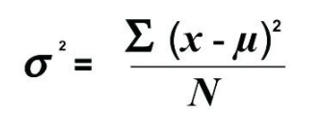
As you explore this formula, first notice the symbols it uses. We discussed µ and N as representing population values. We also designate the population variance with σ2 (sigma squared).

To compute the variance, we take the difference between each value (x), and the population mean, µ. Then, we square each difference, sum up the squared differences, and then divide the sum by N, the number in the population.

To see how this works, we will assume the quiz scores we have been using represent a population. To compute the variance, we take the following steps:

1. Compute the population mean. (100+68+68+68+67+67+66)/7 = 72 – we use µ to represent the mean because we are considering this a population, not a sample.

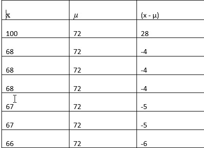
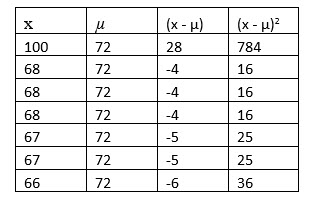
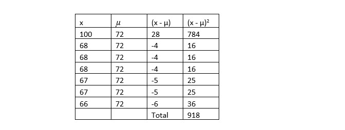
2. Compute the difference between each value and the mean:

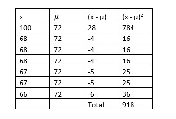
3. Square the differences between x and µ.

This formula is =B6-B9.

4. Divide the sum of the squared differences by the number in the population, N.

918 / 7 = 131.1429 so, the population variance is 131.1429.

The computed variance of 131.1429 may seem large considering the values we started with. Remember, this is the mean of the squared differences (deviations). Notice the deviation from the mean for the highest value, 100. It has a large deviation which results in a very large squared deviation. We discussed this value as an outlier that affected the mean. Outliers also cause the variance to be larger. But that is exactly why we compute the variance. The variance we computed tells us there is a large dispersion or variance in the values of these exam scores.

Sample variance:

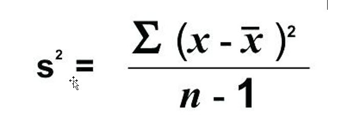
At first glance, the sample variance formula appears quite different than the population variance. However, when we remember that samples use different symbols, there is truly very little difference. Let’s look at the same and different portions of this formula.

First, notice that sample variance is designated with s2 rather than σ2. The other symbol to notice is x̅, which represents sample mean rather than population mean. So, the sample variance begins with the sum of the squared differences between each value and the mean, sample mean in this case. However, the real difference between the sample and population variance is the denominator. Rather than dividing the sum of the squared differences by the number in the population, N, we divide by one less than the number in the sample, n – 1.

We will use the quiz scores to compute sample variance. We will assume the seven students represent a subset of a larger statistics class. To compute the variance of the exam scores, we take the following steps:

1. Compute the sample mean, x̅. (100+68+68+68+67+67+66)/7 = 72 – we use x̅ to represent the mean because we are considering this a sample.

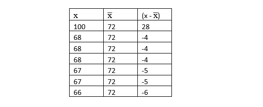
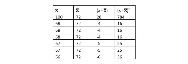
2. Compute the difference between each value and the sample mean, x̅:

3. Square the differences between x and x̅.

4. Sum the squared differences.

5. Divide the sum of the squared differences by one less than the number in the sample, n - 1.

918 / 6 = 153 so, the sample variance is 153.

You may notice the sample variance is larger than the population variance. Of course, this makes sense when you remember you subtracted 1 from the sample size, making the denominator smaller. The official reason for subtracting 1 from the sample size is to reduce potential error (bias) from the values computed from samples, (statistics), and the population parameters.

Try it in Excel:

It is a good idea to understand how to compute the variance on your own, so you are familiar with how this computation works. Of course, Excel has built-in functions to compute both the sample and population variance.

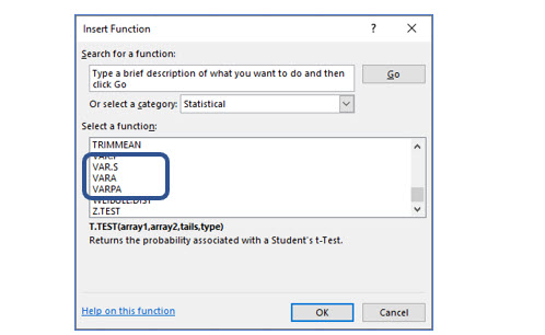
Within Excel’s Statistical function category, you will find the VAR.P and the VAR.S functions. The “P” of course stands for population and the “S” for sample.’

As you can see in the figure below, the values Excel computed matched our computations for both the population and sample variance.

STANDARD DEVIATION:

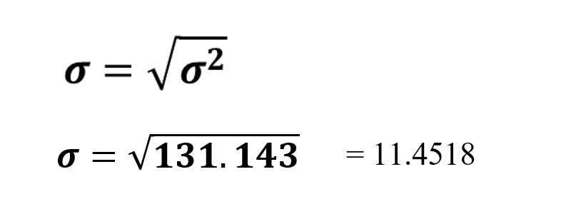
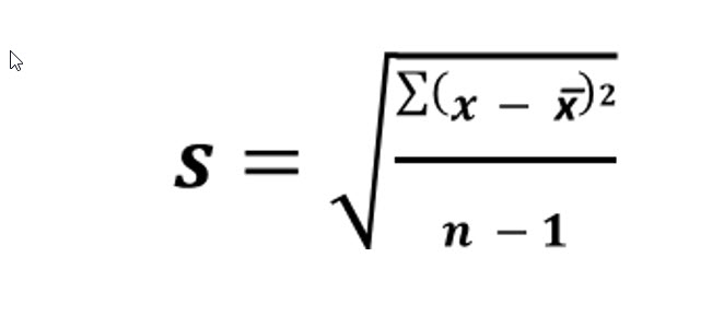
In common statistical usage, the standard deviation is used more often than the variance. Once you have computed the variance, computing the standard deviation is very easy. The standard deviation is the square root of the variance.

Population Standard Deviation:

Sample Standard Deviation:

This formula is =B6-B9.

Try it in Excel:

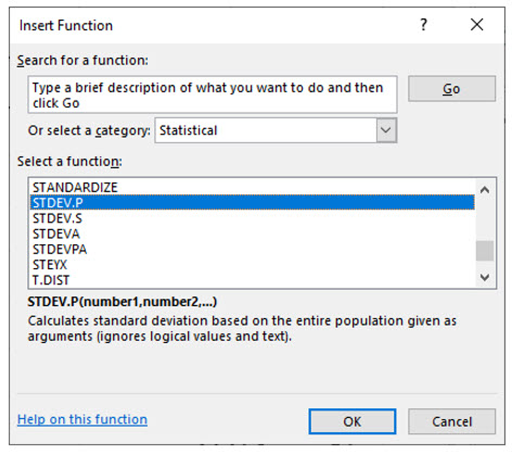
Excel has built-in functions for population standard deviation and sample standard deviation. You can find these functions in the Statistical category.

As you progress in statistics, you will find that you are using the standard deviation frequently. As you interpret data based on the standard deviation, you will find that a relatively small standard deviation indicates that most of the data points lie rather close to the mean.

THE EMPIRICAL RULE

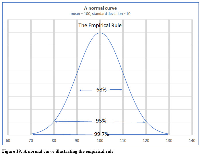
You will spend considerable time in your statistics class dealing with data distributed within a normal, bell-shaped curve. In a normal curve, the highest point is the mean and, within a normal distribution, most of the observations will fall near the mean.

The empirical rule allows you to quickly “guestimate” how many of the observations fall within certain values. For example, using the illustration of the normal curve in Figure 19, the mean is 100 and the standard deviation is 10. The empirical rule tells us that 68% of the observations fall within + or – one standard deviation of the mean, or between 90 and 110 in this example.

The empirical rule also states that 95% of the observed values will fall within + or – two standard deviations, or with this example, between 80 and 120. Almost all, 99.7% of the observed values will fall between + or – three standard deviations of the mean, or between 70 and 130 here.

So what’s the big deal?

Using the empirical rule, we can estimate values that will appear in data sampled from the population. In other words, knowing that 95% of the data points fall within + or – two standard deviations of the mean, we could sample someone in this population completely at random and be 95% sure their value was between 80 and 120.

Even though we are still working with descriptive statistics officially, you may be able to see how the empirical rule could help us begin to infer things about our data. If we know the mean and standard deviation, then we can guess a range of values and be accurate up to 68%, 95%, or 99.7%, depending on the level of accuracy we need and the number of standard deviations we are willing to extend beyond the mean.

Sponsored Ads

---