Chapter 1: Introduction to Statistics and Essential Terminology

This chapter in Surviving Statatistics lays the foundation for all upcoming chapters. It covers quantitative and qualitative vairables, measurement scales and other important foundational concepts.

Note: This chapter is excerpted from Luther Maddy’s Surviving Statistics textbook (C) 2024 which is available in printed or eBook format from Amazon.com

Instructional Videos

Surviving Statistics: Terminology

Business Statistics: Intro & Terminology

Statistics Defined

A statistics guide or textbook should start by defining “statistics”. So, what is statistics? Or, should the question be what are statistics?

Both questions are correct. And so, the confusion begins right on the first page.

Here is an attempt to clear up the definition.

Two Definitions of Statistics

1. Statistics IS the science (branch of mathematics) that deals with collecting, organizing, analyzing, presenting, and interpreting data (mass quantities of numbers), most often to assist decision making processes.

2. Statistics ARE organized, analyzed, presented, or interpreted quantitative data (numbers).

So, you use statistics to produce statistics.

As you move through this book, this will make more sense. Trust me for now.

Another definition I like: Statistics is the process of producing useful information from raw data.

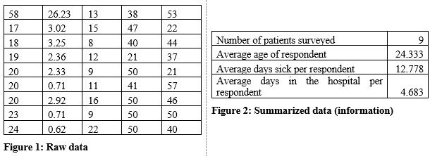
Which figure above makes more sense? Of course, it is Figure 2 with the summarized information. Raw data is important, but it becomes more useful after we use statistics, (the process of summarizing, and presenting data) to display some statistics (organized and summarized information) based on that raw data.

Two Categories of Statistics

While they are both considered statistics, there are two types of statistical information you will compute: descriptive and inferential.

DESCRIPTIVE STATISTICS

As the term implies, descriptive statistics describe the data. A descriptive statistic may be a simple as counting the number of people in a classroom. Descriptive statistics can move up the scale of difficulty and include computations like average, variance, standard deviation, skewness, and beyond. You will become familiar with these terms if they are new to you now. The important point is to understand that descriptive statistics describes the data.

INFERENTIAL STATISTICS

As this term implies, inferential statistics result in inferences, decisions, predictions or estimates. Think about an election. Before the election, if you watch or listen to the news, you would probably hear pundits predicting the likely winner. These pundits are making their predictions based on statistics. You may even hear them throw out percentages such as, “there is a 95% chance that Candidate A is going to win.”

Inferential statistics are an important part of introductory statistics. Descriptive statistics are useful, but they simply describe what is. Inferential statistics try to predict, or infer, what might be, based on statistical information.

Researchers (and students in their statistics courses) use inferential statistics to make inferences, predictions, decisions, or estimates for populations based on data we or others have gathered from samples.

It may be time to define two of the terms I just used.

Population vs Sample

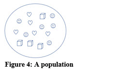
A population includes every person, or object in whatever group is being studied. For example, a population might be every car on a particular car lot or every student attending a college. Populations can be quite large, such as every person residing in the United States, but they do not have to be large. For instance, we might consider every student attending specific statistics course a population.

Now, back to inferential statistics. Let’s assume you want to know how many “happy faces” there are in the example population in the illustration. Answering that question is easy. Just count them. But this gets trickier.

Assume you want to know the makeup of this population. More specifically, you want to know the ratio of happy faces to the entire population. Or, you need to find the percentage of the entire population that are happy faces.

Answering these two questions requires you to look at (survey) every shape in the population in Figure 4. You will need to check every shape in the population to see if it is a happy face. You also need to examine and count every shape so you can find the total number of shapes in the population as well as the number of happy faces. The answer that you should have computed by now is 6/15 or 40%.

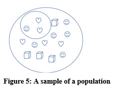
A sample is a representative portion, a subset of a population. Figure 5 illustrates a sample of three symbols from the population of 15 symbols. Inferential statistics, as we stated earlier, makes inferences, predictions, decisions, or estimates for populations based on data gathered from samples.

Using the sample from the illustration, the percentage of happy faces is 1/3, or 33.3%. Based on this sample we might infer that the ratio in the population is also 1/3. In this case, the percentage of happy faces in the sample is not quite the same as the percentage in the population. We will deal with that issue later.

WHY WORK WITH SAMPLES?

As we just saw in the previous paragraph, a sample may lead to an incorrect assumption (inference) about the population. If a sample may not be an accurate representation, why take a sample instead of surveying the population?

First, let’s briefly address the accuracy issue. You will learn in later chapters that samples can and do provide an accurate way to make inferences about populations. You will also learn how to deal with potential inaccuracies. For now, we will assume that samples can be accurate representations of a population.

Reasons to use samples instead of the entire population vary but include:

• Surveying the entire population would be expensive and time consuming. Consider a population as large as every resident in the United States. Surveying every individual in the country would be expensive and time consuming. The United States only attempts to do this once every ten years with the US Census.

• Sometimes surveying or testing is destructive. Suppose you oversee quality for a candy bar manufacturer. To test the quality, you have to unwrap the bar and taste it. Selling candy bars would be very difficult to sell your candy if every candy bar is unwrapped and has your teeth marks in it. Sampling is a better choice.

Variables

Surveying or testing a sample or a population involves asking questions, testing, or measuring. In your survey or test, you are interested in certain values or characteristics. Those values or characteristics are variables. For example, if you are studying basketball teams, you may decide to measure the height of each player. In this case, height would be considered a variable. There are two broad categories of variables: quantitative and qualitative.

QUALITATIVE VARIABLES

ualitative variables are nonnumeric

Assume you still work at the candy company received a promotion. Now you are doing market research for your employer. You are a basketball fan, so you decide to survey the players on your college’s team about their favorite candy bar. Their favorite candy bar is a qualitative variable because it is not a number.

Continuing with your survey, you ask each player to explain why a particular candy bar is his or her favorite. The answer to your “why” question is also a variable. If the player was particularly passionate about their favorite candy bar, this variable could be several paragraphs of text. Not unimportant, just lengthy.

QUANTITATIVE VARIABLES

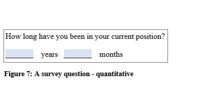
Quantitative variables are numeric. These might be measurements of height, weight, test scores, or income. Quantitative variables can also be counts such as how many children are in a family, how many cars are in a parking lot, or how many students are absent from a class.

Since statistics, (i.e. the process) deals with numbers, (i.e. statistics) it may be obvious that we will be dealing with quantitative variables more often than qualitative variables.

For instance, if a survey variable was “favorite color,” how would you compute an average of the sample’s favorite color?

Using Qualitative Variables in Statistics

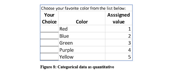
Do not give up on qualitative variables entirely because we can use them in statistics. However, we must first convert them into quantitative variables. For example, we could convert the choice of favorite color into a number. You could assign a value of 1 to red, 2 to blue and so on. You can also do something similar with the variable “gender” or other qualitative variables. Qualitative variables that can be converted into numerical data are called categorical variables.

While some qualitative variables can be converted to numbers, others are more difficult. Think about the variable, “Why do you like your favorite candy bar?” Since the answers can vary greatly, it would be very difficult to convert it into a numeric value. Qualitative variables like the “why” question are useful, just not in statistical analysis. (There are tools and techniques to help make sense of and analyze qualitative variables in research, but that is not something for this course. You will learn about these tools in a qualitative research methods course.)

Types of Quantitative Variables

As you have probably guessed, the statistical process is concerned with quantitative variables. So, we now need to discuss two main types of quantitative variables and four measurement scales we use to classify them.

Discrete variables result from counting. The number of students enrolled in a class, the number of devices connected to the internet in a home, and the number of patients in a hospital are examples of discrete variables.

Continuous variables are measured rather than counted and can assume any value for the item being measured. The weight of patients entering a hospital, the amount of time it takes students to complete an exam, and the amount of gasoline in your tank are all examples of continuous variables.

Four Quantitative Measurement Scales

Quantitative variables are classified into one of four measurement scales. The scale we use controls what types of statistical analysis we can perform with that variable.

To introduce this concept, consider two variables, the heights of basketball players on a team and numeric values assigned to a favorite color choice. Counting how many people like red and how many like blue would be useful. However, computing an average of the sample’s favorite color would be worthless. Blue and a half, makes no sense. On the other hand, the average height of a basketball player is very useful. The scale a variable uses limits the statistical computations that are useful. The four scales used for quantitative variable are nominal, ordinal, interval, and ratio.

NOMINAL SCALE

A nominal scale is used for data than can be categorized and assigned values, but those values do not equate to relative worth or order. Again, think about the variable for favorite color assigned values. While you may prefer blue, that color is not more valuable or better than any other color. So, assigning red a value of 1 and blue a value of 2 does not mean that either has more relative value than the other. Beyond counting and computing percentages, statistical analysis of data that uses a nominal scale is very limited.

ORDINAL SCALE

Data that uses an ordinal scale can be ranked or ordered in a meaningful way. However, the differences between items in the ranked list either cannot be determined or are not meaningful. For example, you can list your favorite, next favorite and third favorite ice cream flavors as 1, 2, and 3. The order is important, you cannot numerically determine how much you like flavor #1 more than flavor #3. As with nominal scale data, analysis is limited to counting and percentages with variables using the ordinal scale.

INTERVAL SCALE

The interval scale is used for data with meaningful and measurable differences between values. Many additional statistical computations can be performed with data using the interval scale than can be performed with data using the nominal or interval scales. One of the identifying attributes of the interval scale is that zero does not really indicate a null value. The classic example of the interval scale is temperature. Neither 0oC or 0oF equates to the absence of temperature. Some clothing items, such as ladies’ dresses and infant shoes also use the interval scale. A shoe size of zero does not mean the absence of any shoes.

RATIO SCALE

The major attribute that sets the ratio scale apart from the interval scale is that zero does mean zero. Both discrete and continuous variables can be measured using the ratio scale. One example of a discrete variable measured with the ratio scale might be the number of students in class on a particular day. In this case, zero means no students attended. A continuous variable using the ratio scale might be the amount of income taxes paid or the amount of gas in your tank.

Sponsored Ads

---