Gooodness of Fit tests

This chapter explains computing the goodness of fit for equal and unequal frequency distributions.

Note: This chapter is excerpted from Luther Maddy’s Surviving Statistics textbook (C) 2024 which is available in printed or eBook format from Amazon.com

Instructional Videos

Surviving Statistics: Goodness of Fit tests Business Statistics: Goodness of Fit tests

Surviving Statistics Chapter 14- File Downloads

Fast Food Preferences

Goodness of Fit Tests

Goodness of fit tests allow us to do hypothesis testing on data that uses the nominal scale of measurement. As we discussed in the first chapter, we cannot compute means and several other measurements from data that uses the nominal scale. We can, however, measure and analyze frequencies or counts. In this chapter, we will be discussing goodness of fit tests, which compare actual frequencies to the counts we expected. We will be using the chi-square, X2, statistic in this process.

Goodness of Fit – Equal Expected Frequencies

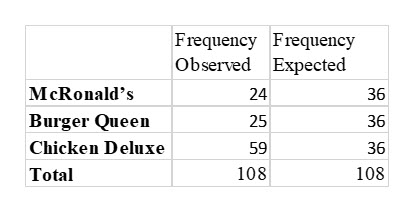
Tina thinks all fast food is the same. In her opinion, one franchise is just as bad as another. Tina also believes that everyone feels the same way. She is sure no one she surveys will express a preference for one fast food vendor over another. She sets out to test her hypothesis by randomly surveying 108 people. She asks them to pick their favorite fast-food provider from a list of three popular establishments. Tina recorded the following results:

Step 1: State the null and alternate hypothesis:

H0 There is no difference in the preference of fast food vendors. H1 There is a difference in the preference of fast food vendors.

Step 2: Select the level of significance:

Tina selects a .05 level of significance, giving her a 5% chance of making a Type I error.

Step 3: Determine the test statistic:

The goodness of fit uses the X2, chi-square, distribution.

Step 4: Determine the critical value (decision rule):

The degrees of freedom for the X2 distribution are k – 1. In her survey, Tina has three categories, fast food vendors, so the degrees of freedom are 2.

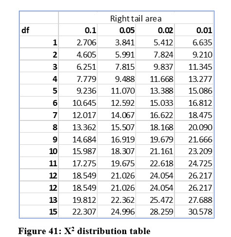
Locating the .05 right tail area (like the F distribution, the X2 cannot be negative and therefore only has the right tail), with 2 degrees of freedom results in a critical X2 value of 5.991 as shown in Figure 41.

Step 5: Take a sample, compute the test statistic and make a decision

The expected frequency is needed to compute the X2 statistic. In this case, since Tina expected there to be no preferences. So, the frequency expected for each vendor is the same, 36, (108/3).

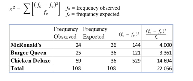
The formula to compute the X2 statistic is:

Tina’s computed X squared statistic is larger than the critical value and is in the rejection area. At a significance level of .05, Tina rejects the null hypothesis which was her belief that there is no preference for one fast food restaurant over another. Tina has learned that perhaps some people do like fast food, or at least prefer the establishments they frequent.

Goodness of Fit – Unequal Expected Frequencies

A recent study conducted by the Chicken Growers of America, found that people prefer chicken sandwiches to burgers on a 2 to 1 ratio. Hearing this, Tina is still not convinced that anyone could really have a preference for any type of fast food. She sets out to use her previously collected data to prove this study wrong.

Step 1: State the null and alternate hypothesis:

H0 There is no difference between the results reported by the chicken growers and the results of Tina’s survey. H1 There is a difference between the results reported by the chicken growers and the results of Tina’s survey.

Step 2: Select the level of significance:

Tina selects a .02 level of significance, giving her a 2% chance of making a Type I error. She is sure selecting this level of significance will strengthen her campaign to stamp out fast food, if her hypothesis proves to be correct.

Step 3: Determine the test statistic:

The goodness of fit uses the X squared, chi-square, distribution.

Step 4: Determine the critical value (decision rule):

The degrees of freedom for the X2 distribution are k – 1. In her survey, Tina has three categories, fast food vendors, so the degrees of freedom are 2.

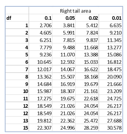
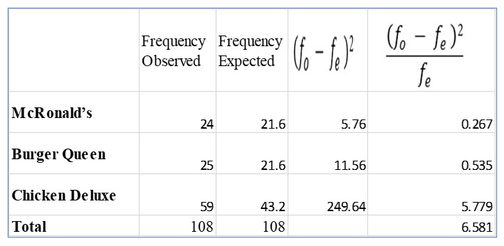
Locating the .02 right tail area with 2 degrees of freedom results in a critical X squared value of 7.824.

Step 5: Take a sample, compute the test statistic and make a decision

Tina’s computed X squared statistic, 6.581is not larger than the critical value, so it is in the “do not reject” area. Once again, Tina’s assertions have not proven to be true. She cannot reject the null hypothesis and her research seems to agree with the Chicken Growers data.

Tina gives up on her research and decides to try a sandwich from Chicken Deluxe.

Sponsored Ads

---