Correlation and Linear Regression

More Statistics Topics
Correlation and Linear Regression

Correlation and Linear Regression

This chapter explains computing the Correlation Coefficient, dependent and independent variables and performing linear regression manually and with Excel.

Surviving Statistics: Correlationn & Regression Business Statistics: Corelation and Linear Regression Business Statistics: Multiple Regression Analysis

Surviving Statistics - File Downloads

Lemonade Sales

Correlation and Linear Regression

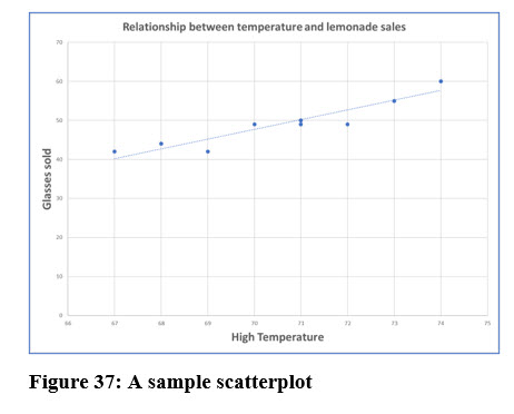
You may recall the scatterplot we discussed in Chapter 4 as shown in Figure 37. The purpose of a scatterplot is to display a possible relationship or correlation between two variables. The scatterplot shown below displays the relationship between the amount of lemonade Larry sold and the day’s high temperature. We also briefly introduced you to the concept of a numerical value that represents the same thing, the correlation coefficient.

In this chapter, we will compute the correlation coefficient that indicates the relationship strength between two variables. We will use linear regression to attempt to determine the relationships between variables and predict values for one variable based on the values of one or more other variables.

Dependent and Independent Variables

Both correlation and regression analysis deal with dependent and independent variables. Independent variables are usually designated as X and dependent variables are designated with Y. In the lemonade stand example, the scatterplot seemed to indicate that lemonade sales were affected by the temperature. With linear regression, we are attempting to predict values of the dependent variable, Y, based on values of the dependent variable, X.

Correlation Coefficient

The correlation coefficient measures the strength of the linear relationship between two variables. Its value can be negative or positive and ranges from -1 to +1 as shown in Figure 38. In the lemonade stand example, the scatter plot suggests a strong positive correlation between the high temperature and the amount of lemonade sold.

The formula to compute a correlation coefficient is:

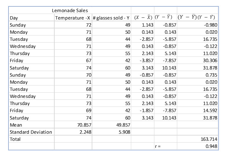
The computations for Larry’s lemonade are as follows:

The computed correlation coefficient of .948 confirms our observation from the scatterplot. There is a very strong positive relationship between the day’s high temperature and lemonade sales.

Regression Analysis

The result of regression analysis is an equation that we can use to predict a value for a dependent variable based on independent variable(s). Linear regression rests on the least squares principle, which creates a line minimizing the sum of the squares between the actual and predicted values of Y, the dependent variable.

The linear equation will have an intercept and a slope. After computing the slope and intercept you can then use various values of X, the independent variable, to predict value for Y.

The linear regression formula is:

SLOPE

The slope determines how much Y increases with each increase in X. The formula to determine the slope is:

We have already computed the correlation coefficient, r for the lemonade sales example. We have also previously computed the standard deviation for both variables. So, we can compute the slope as:

INTERCEPT

The Y intercept, the value of Y when X = zero is computed as:

As with the slope, we have everything we need to compute the intercept as:

REGRESSION FORMULA

Now that we have computed the slope and intercept, we can complete the regression formula as:

So, if the high temperature of the day is going to be 75 degrees F, we would predict Larry would sell:

Predicted glasses sold = -126.687 + 2.49145(75) = 60.18

Try it in Excel:

Computations for regression analysis can be time consuming to do manually. Statistical software and Excel make them much easier. We’ll go over the steps to perform regression in Excel and discuss some important regression analysis parameters which Excel includes in it summary output table.

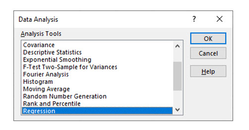
In Data Analysis, choose Regression.

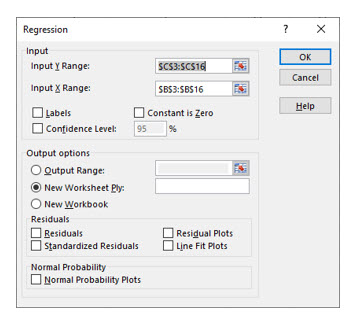
Next, highlight the cells for the Y (dependent variable) and the X (independent variable) and click OK.

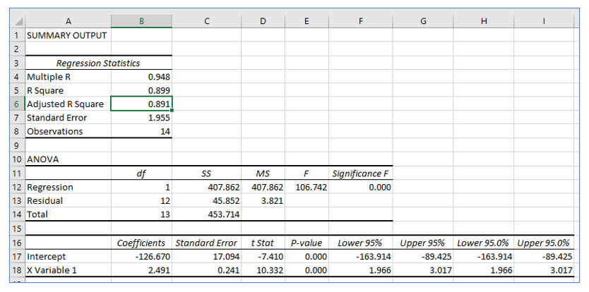
The intercept we computed, -126.670, appears in this output in cell B17.

The slope, 2.491, appears in cell B18.

From these two cells, you can create the regression equation.

Notice that Excel also computed the correlation coefficient, r in cell B4. Excel names it “Multiple R,” but it is still the correlation coefficient.

STANDARD ERROR OF THE ESTIMATE

The standard error of the estimate measures how widely the predicted values and actual values are dispersed. The larger the standard error of the estimate, the more the actual data points vary from the created regression line (predicted values). If you use Excel or other statistical software to compute a regression, this value is calculated for you. You can see the standard error in cell B7 of the regression output.

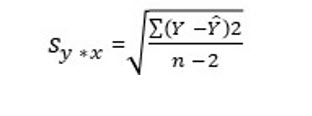
The formula to compute the standard error of the estimate manually is:

COEFFICIENT OF DETERMINATION

The correlation coefficient, r, measures the strength of the relationship between the dependent and independent variable. The coefficient of determination, r2, measures the proportion of variance in the dependent variable, Y, that can be explained by the dependent variable, X. The coefficient of determination is computed by simply squaring r. In the regression output, the coefficient of determination shown in cell B5 is .899. This tells us that roughly 90% of the variability in lemonade sales can be explained by the day’s high temperature.

Multiple Regression

In Larry’s lemonade example, we examined the relationship between sales and one independent variable, the day’s high temperature. However, Larry thinks there may be other factors that affect lemonade sales. The purpose of multiple regression is to create a regression equation that more accurately predicts values of the dependent variable because it includes additional statistically significant independent variables.

Continuing on with Larry’s Lemonade, Larry believes he sells more lemonade when the humidity is higher. He also believes he sells less lemonade on days on which rain is likely. He also thinks he sells more lemonade on workdays than he does on the weekend.

In creating a multiple regression Larry, or whoever does the analysis, will throw every possible variable into the mix. Then, after the regression is computed, each potential independent variable will be evaluated to see if it is a statistically significant predictor of the dependent variable. Variables that are not statistically significant predictors are eliminated from the regression equation and the result is an equation that can accurately predict the independent variable.

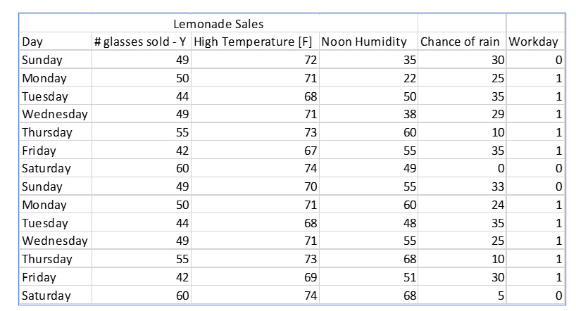
The next figure shows the data Larry has collected to analyze in a multiple regression.

DUMMY VARIABLES

You may notice that Workday has a value of 0 or 1. Workday is a qualitative variable, not quantitative. Dummy variables allow some qualitative variables, those that use a nominal scale to be used in regression. In this case workdays are coded as 1 and weekend days as 0.

Performing a multiple regression is very difficult to do manually. We will illustrate this example using Excel and discuss its output.

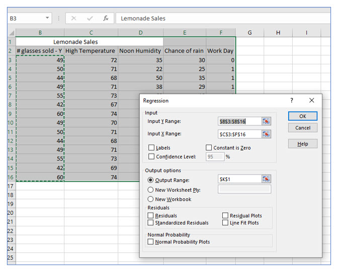
When performing a multiple regression in Excel, highlight all the potential dependent variables in the X range.

THE MULTIPLE REGRESSION EQUATION

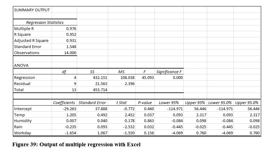
From Excel’s regression output in Figure 39, we can easily create a multiple regression equation. The illustration shows the names of the variables. By default, Excel labels the X Variable 1, X Variable 2, and so on.

The multiple regression equation, before we evaluate it is:

Predicted Lemonade Sales = -29.263 + 1.205(Temp) + .007(Humidity) - .235(Rain) – 1.654(Workday)

EVALUATING A MULTIPLE REGRESSION OUTPUT

Correlation Coefficient

As we examine the output from Excel’s multiple regression output, we first examine the correlation coefficient, r. Excel labels this “multiple R” and has computed this as .976 and this indicates a very strong positive correlation between lemonade sales and all the variables included in the multiple regression.

The Global (F) Test

The global test measures whether or not ALL the slopes of the independent variables are zero. This is actually a hypothesis test and the null hypothesis is that all of the slopes are zero, or not significant predictors of the dependent variable. The alternate is that at least one is not zero, and therefore, at least one is a significant predictor. (Because we already performed a single regression. We already know that temperature is a significant predictor, so we are actually only concerned about the others.)

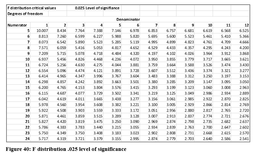
To determine the critical value for F with a .05 level of significance, we use 4 degrees of freedom in the numerator, computed as p (number of all Y and X variables) – 1. The degrees of freedom for the denominator are 9, computed as n – p. Notice that Excel displays the degrees of freedom in its output.

The critical value from the table in Figure 40 is 4.718. Remember we divide the level of significance by 2 with the F distribution. The F statistic that Excel computed for this example is 45.093. This is far larger than the critical value, so we will reject the null hypothesis and conclude that at least one of the independent variables included in the analysis is a significant predictor. In practice, we don’t have to locate the critical F values if we are using Excel. Instead, we can use the p value Excel labels “Significance F”. The p value is essentially zero in this example, which makes sense when we see how large the computed F is in relation to the critical value at the .05 level of significance.

Because we have rejected the null hypothesis in the Global test, we will continue to evaluate the variables.

Evaluating Each Independent Variable

The Global test lets us know that at least one of the independent variables is a statistically significant predictor of Larry’s lemonade sales. The next step is to evaluate each variable to see if it should be included in the regression equation. We can do this by testing the slope of each variable with a t test.

The evaluation process is also a hypothesis test. The null is that the slope is zero, which would mean it is not a significant predictor. The alternate is that the slope is not zero and is therefore, a significant predictor of the dependent variable. In this example, we will use the .05 level of significance.

This is a two-tail test. We compute the degrees of freedom as n – (k + 1), where n (number of observations) = 14 and k is the number of independent variables. The result is 9 degrees of freedom. We can see that Excel computed this for us and the result is the same as that for the denominator of the global F test, n – p. The critical t value with 9 degrees of freedom is 1.833. You can use the table in Figure 36 on page 129 to verify this value. Knowing the critical value, we can then compare the t stat for each independent variable and determine if it is a significant predictor of lemonade sales.

The t values Excel computed are as follows:

Temperature = 2.452 Humidity = 0.178 Rain = -2.532 Workday = -1.550

From the t values, we know that only temperature and rain are significant predictors of lemonade sales. The other variables, while they may play some part in lemonade sales, do not pass the test based on the criteria Larry established, the .05 level of significance.

Rather than going to all the effort of computing the degrees of freedom and looking up the critical t value, Larry could have simply used the p values that Excel displays in its regression output for each of these variables. In Excel’s output only temperature and rain have p values that are <= .05, the level of significance Larry established.

Creating a More Accurate Multiple Regression Equation

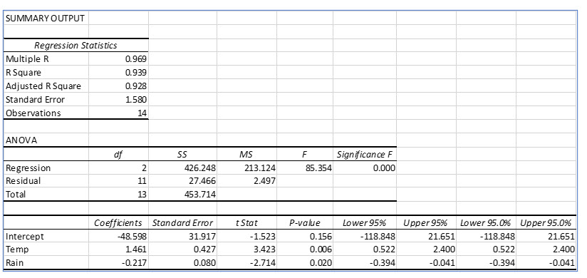
Larry threw every possible independent variable he could think of into the multiple regression. Not all the variables he included proved to be statistically significant predictors at the .05 level of significance. The next step is to run another regression, but this time only including the two significant predictors, temperature and rain.

In the new regression the global test (F), is larger than the previous regression and the p value for the F test is essentially zero. This lets us know that at least one of the independent variables included in this regression is a significant predictor. (But we already knew that.)

The new regression model more accurately models the data than the first regression which included variables that were not statistically significant predictors of lemonade sales. You should also notice that the t values are larger, and the p values are smaller than the first regression. Now, we can create a multiple regression equation that includes only significant independent variables. The revised multiple regression equation becomes:

Predicted Lemonade Sales = - 48.598 + 1.461(Temp) - .217(Rain) For a high temperature of 800F and a 40% chance of rain, - 48.598 + 1.461(80) - .217(40) = 62.602 lemonade sales