ANOVA (Analysis of Variance)
This chapter in Surviving Statatistics explains how to complete an Analysis of Variance when working with two populations or more than two samples.
Note: This chapter is excerpted from Luther Maddy’s Surviving Statistics textbook (C) 2024 which is available in printed or eBook format from Amazon.com
Instructional Videos
Surviving Statistics: Analysis of Variance - ANOVA
Business Statistics: Analysis of Variance - ANOVA
Creating an ANOVA table in Excel
Surviving Statistics Chapter 12 - File Downloads
Patient Discharge Times ANOVA table
ANOVA (Analysis of Variance)
We use the ANOVA to compare the variance of two populations or to compare the means of more than two samples. We accomplish these two goals differently, but both will use a test statistic we have not yet used, the F statistic
Here are some attributes of the F distribution you should know:
• The F distribution, like the T distribution uses degrees of freedom.
• The F statistic will never equal a negative value, but it can be zero.
We will start this chapter with a comparison of two population variances and a simple formula to compute the F statistic. Then we will create a complete ANOVA table as we compare the means from three samples.
Comparing two population variances
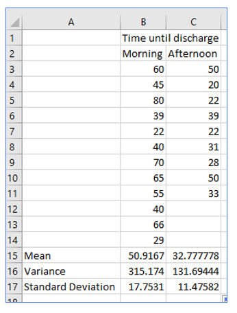
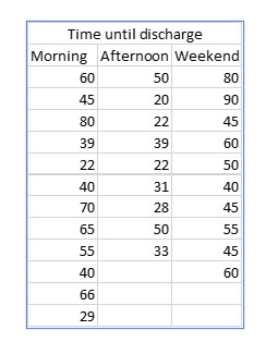
Although it does not appear on every patient satisfaction survey, Keisha keeps running into one consistent complaint: the discharge process takes too long. Patients comment that the waiting time after the doctor releases them to when they can actually leave the hospital is too long. Keisha wants to compare the dispersion (variance) in times between patients released by their doctors before noon and those released after noon. She decided to compare the variances of these two populations. To do this, she surveyed a sample of 12 patients released in the morning and 9 patients released after noon. The results are as follows:
Step 1: State the null and alternate hypothesis:
H0 Variance of morning releases = Variance of afternoon releases
H1 Variance of morning releases <> Variance of afternoon releases
Step 2: Select the level of significance:
Keisha selects a .02 level of significance. This gives her a 2% chance of making a Type I error.
Step 3: Determine the test statistic:
Because Keisha is comparing the variances of these two populations, she will use the F distribution.
Step 4: Determine the critical value (decision rule):
This is a two-tail test because Keisha is checking both directions, which means Keisha is looking for .01 in each tail. Even though the F distribution does not support negative values, we will still treat this as a two-tail test.
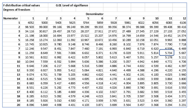
The F distribution uses two degrees of freedom, one for the numerator and one for the denominator. The numerator will be the sample size of the sample with the largest variance, and the denominator is the size of the sample with the smallest variance.
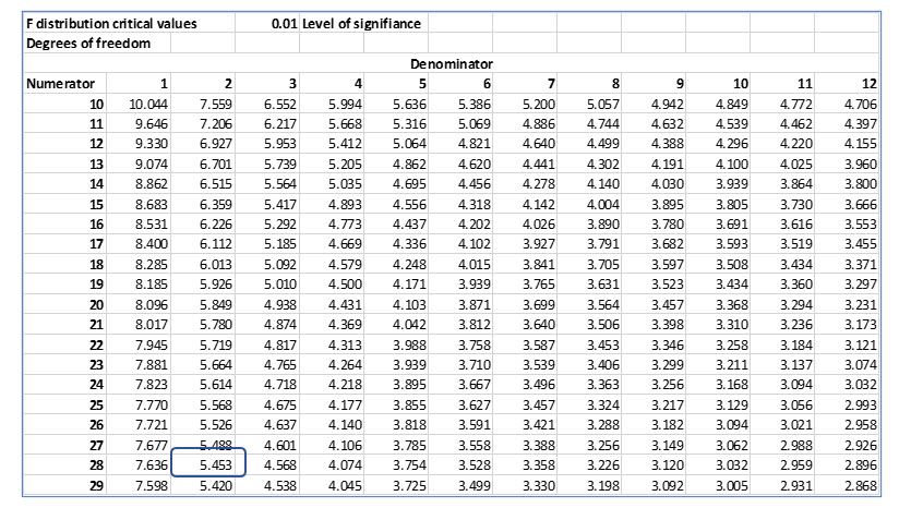
The degrees of freedom for the numerator and the denominator are n – 1, so 11 for the numerator and 8 for the denominator. Locating the .01 table and the degrees of freedom for the numerator and denominator, the critical F value is 5.734.
Step 5: Take a sample, compute the test statistic and make a decision
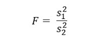
Keisha has already taken the sample, so the next step is to compute the F statistic. The formula to do this is:
Keisha computes an F of 2.393. Since this F statistic is smaller than the critical value, Keisha does not reject the null hypothesis. Even though the variances appear to differ, she cannot conclude that is actually the case at the .02 significance level.
If Keisha is uneasy with these results, she could conduct another study with a larger sample size. Notice the critical values in the F table decrease substantially as the degrees of freedom increase. With a larger sample size, Keisha’s decision could be different.
Completing an ANOVA table – three or more means
The t test works well for comparing two sample means. However, it becomes very tedious to use the t statistic to compare three or more means. The ANOVA is a better approach. The final result of the ANOVA will be an F statistic that can be used to reject or not reject the null hypothesis. When we are comparing three or more means the null hypothesis is that the means are equal. The alternate is that at least one mean differs from the others. (Theoretically, we are testing if the means of the populations that the samples were taken from are equal.)
Software programs, like Excel and specialized statistical applications, make creating an ANOVA table quick and easy. However, we will step through the manual creation process first to help you better understand the values that the ANOVA table displays. We will also use ANOVA tables in upcoming chapters.
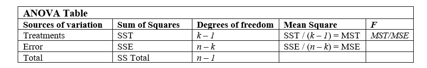
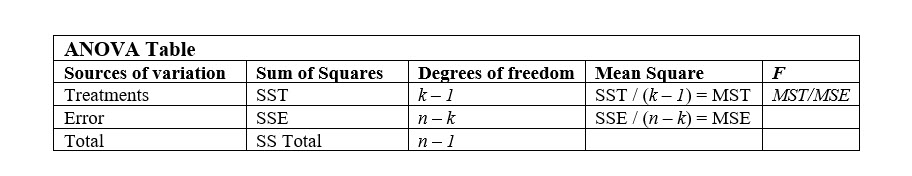
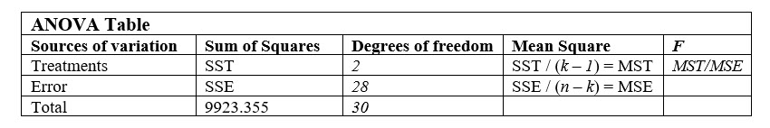
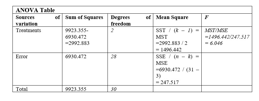
Before we begin the five-step hypothesis testing process, here is an illustration of an ANOVA table and the values we will be computing. This table will make more sense as we step through the process.
Keisha is still interested in the time patients wait after being released by their doctor until they are actually discharged. She wants to compare the average (mean) waiting time for those released by their doctors in the morning, afternoon, and weekends. She wants to know if there is a statistically significant difference in the mean waiting times for these three patient populations.
To test her hypothesis, Keisha collects the following data:
Step 1: State the null and alternate hypothesis:
H0 Mean morning = mean afternoon = mean weekend
Or µ1 = µ2 = µ3
H1 All three means are not equal
Step 2: Select the level of significance:
Keisha will again select a .02 level of significance, giving her a 2% chance of making a Type I error.
Step 3: Determine the test statistic:
Keisha will construct an ANOVA table to compare the means of these three populations with the F distribution.
Step 4: Determine the critical value (decision rule):
This is a two-tail test because Keisha is checking both directions. This means we are looking for .01 in each tail. Even though the F distribution does not support negative values, we will still treat this as a two-tail test.
The degrees of freedom are determined as follows:
Numerator = k – 1 = 3 – 1 = 2
k is the number of categories or populations, 3 in this case.
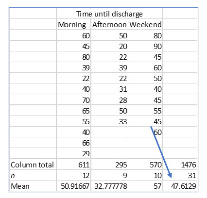
Denominator are n – k = 31 – 3 = 28
n is the total of all three samples which is this case is 31.
The degrees of freedom for the numerator are 2 and the degrees of freedom for the denominator are 28. Locating the .01 table and the degrees of freedom for the numerator and denominator, the critical F value is 5.453.
Step 5: Take a sample, compute the test statistic and make a decision
Keisha has already taken the sample, so the next step is to construct the ANOVA table and compute the F statistic.
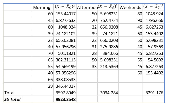
The first step in creating the ANOVA is to create the grand mean, the mean of all the samples. For these samples, the grand mean is 47.613 (1476/31).
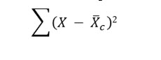
The next step is to compute the Sum of Squares Total (SS Total).
This is computed as:
To compute SS Total, we subtract the grand mean from each value, square it and them sum all the squared differences for each sample.
Completing the ANOVA table as we go, we can now fill it in as follows:
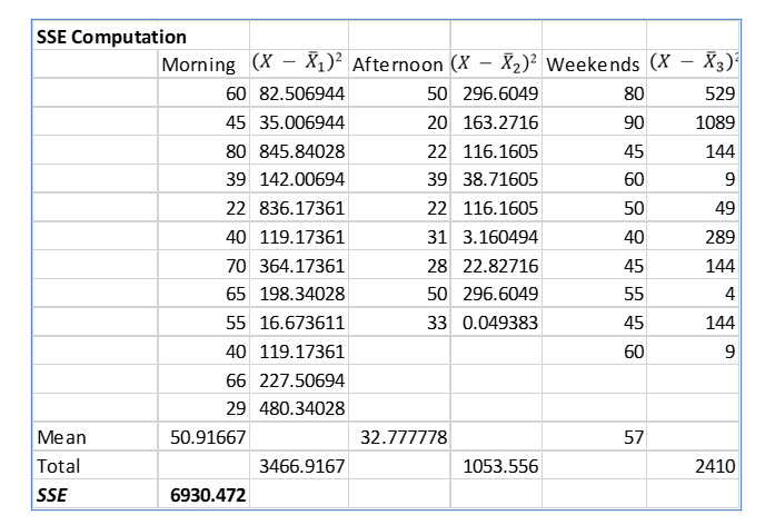
The next step is to create the Sum of Squares Error.
We compute this by taking each value in the sample and subtracting the treatment (sample) mean from that value. We then square the difference for each value and sum all the errors for each treatment (sample). Finally, as the term implies, SSE is the summed treatment (sample) errors.
Once we have these two key values, SS Total and SSE, we can construct the rest of the ANOVA table with minimal calculations.
Having SS Total and SSE, we can easily compute SST with: SST = SS Total - SSE
All the other computations are based on SST and SSE. So, the completed table, including the F statistic is as follows:
After constructing the ANOVA table and computing an F statistic of 6.046, Keisha can reject the null hypothesis because the F statistic she computed is larger than the critical F value of 5.734
All three of the means are not equal at the .02 level of significance. Essentially, Keisha can be at least 98% sure that the wait times in the morning, afternoon, and weekends are not the same.
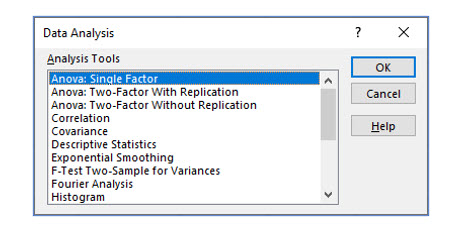
Try it in Excel:
Excel’s data analysis add-in has the ANOVA single factor option that will create an ANOVA table and compute the F statistic for more than two samples.
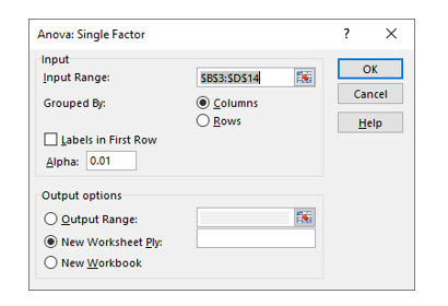
Be sure to set the correct Alpha level, which will be the level of significance / 2 because you are really doing a two tailed test.
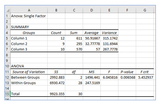
You should be able to understand these values after constructing an ANOVA manually. Notice that Excel names SST, “Between Groups”, and SSE “Within Groups”.