Two sample hypothesis testing

This chapter in Surviving Statistics explains how to complete a Hypothesis testing with two samples.

Chapter Study Sheet

⬇

Printable Study Sheet Open or download

Instructional Videos

Surviving Statistics Chapter 11 - File Downloads

Two sample hypothesis testing

In the previous chapter, we explored hypothesis testing comparing one sample’s mean or proportion to a population mean or proportion. In this chapter, we will discuss the computations needed in hypothesis testing to compare two samples.

Two Sample Hypothesis Testing – Known Population Standard Deviation

We will compare two sample means, each representing a different population. We will, however, need the standard deviation for each population. To help understand this procedure, here is an example.

Keisha, a new administrator for Quad-States Hospital, is interested in the satisfaction ratings for day and evening shift nurses. Patients are asked to rate their nurses on several items on a scale of 1 to 5. As she began her research, she was told that both shifts have equal patient satisfaction ratings and both shifts have a standard deviation of .2.

From listening to a few patients since arriving here, Keisha believes the night shift may be doing a better job caring for patients. She sets out to test this hypothesis.

Step 1: State the null and alternate hypothesis:

H0 Night shift satisfaction ratings <= day shift ratings H1 Night shift satisfaction ratings > day shift ratings

Step 2: Select the level of significance:

Keisha selects a .02 level of significance. This gives her a 2% chance of making a Type I error.

Step 3: Determine the test statistic:

Because Keisha has the historic population standard deviation, she will use the z distribution.

Step 4: Determine the critical value (decision rule):

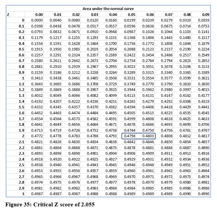
This is a one-tail test because Keisha is only checking one direction. The z score that equates to an area of .48 (2% in the single tail) and using the table in Figure 35, this is close to 2.055.

Step 5: Take a sample, compute the test statistic and make a decision

Keisha randomly surveyed 25 patients and asked them to rate their day shift nurse. She then surveyed another 30 patients and asked them to rate their night shift nurses. The mean for the day shift nurses was 4.55 and the night shift nurses was 4.7.

The formula to compute a z score from two samples is:

Keisha’s computed a z score is larger than the critical value. She will reject the null hypothesis and conclude, at least for this sample, night shift nurses have higher ratings than day shift nurses.

Two Sample– Unknown Standard Deviation

Many times, as we have already discussed, when you are doing your own research you will not have the population standard deviation available. In these cases, you will likely use the t distribution.

To illustrate a two-sample hypothesis test using the t distribution we will revisit Keisha and her hypothesis on nursing ratings. This time though she either does not have the population standard deviation or does not trust the one she was provided.

Step 1: State the null and alternate hypothesis:

H0 Night shift satisfaction ratings <= day shift ratings H1 Night shift satisfaction ratings > day shift ratings

Step 2: Select the level of significance:

Keisha selects a .05 level of significance. This gives her a 5% chance of making a Type I error.

Step 3: Determine the test statistic:

Because Keisha does not have the population standard deviation, she will use the t statistic.

Step 4: Determine the critical value (decision rule):

This is a one-tail test because Keisha is only checking one direction. The t distribution requires Keisha to use degrees for freedom as well as the level of significance to locate the critical value. With two samples, the degrees of freedom are: n1 + n2 – 2, or 53 in this case.

Using a table or Excel, Keisha locates a critical t value of 1.674.

If you examine the Excel formula closely you will notice the (-) at the beginning. Because this function returns the left tail value, which is negative, placing the minus sign at the beginning causes the t critical value to be positive.

Step 5: Take a sample, compute the test statistic and make a decision

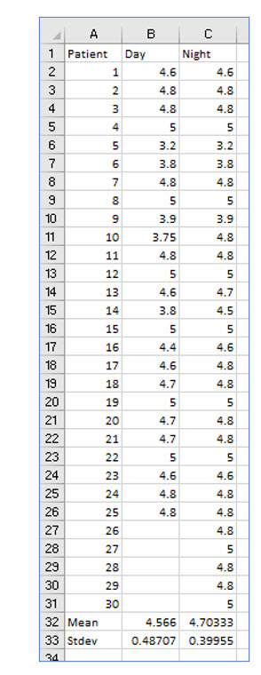
Keisha took two samples, 25 day patients and 30 evening patients. The results with the mean and sample standard deviation are as follows:

Computing a t score from two samples is somewhat complex if you do it manually. Excel has an excellent tool that we will discuss later. For now though, we will go over the manual method.

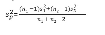
The first step in computing a two-sample t test score is to compute the pooled variance. The formula for doing this is:

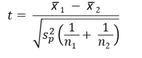
After computing the pooled variance, you use it in the formula to compute a t score, which is:

So, for Keisha, the pooled variance becomes:

The pooled variance = .19478

Notice that we are using the night shift, the sample with the highest mean as sample 1.

Now that we have the pooled variance, we can compute the t statistic as follows:

In this case, the computed t score is less than the critical value, so Keisha will not reject the null hypothesis. She cannot conclude that night nurses receive higher satisfaction scores than day shift nurses do.

When Keisha conducted the first hypothesis test using the z statistic, she was able to reject the null hypothesis. However, using the t test she is not able to do so. This is because the standard deviation she computed with her sample is much larger than the assumed population standard deviation (.02) she used with the z test.

Try it in Excel:

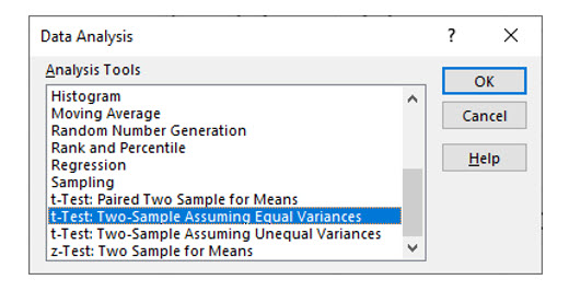
Excel’s data analysis add-in has a t test option that computes the t statistic after selecting the data from both samples. From the data analysis tools, choose t –Test Two sample assuming equal variances.

Note: Even though the variances of the day and night shift samples appear to differ in this example, they are not unequal from a statistical standpoint. In the next chapter, you will learn to conduct a hypothesis test to examine the equality of variance.

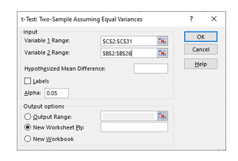
Next, select the two ranges containing the data from each sample. Select the desired alpha level, the level of significance, and click OK.

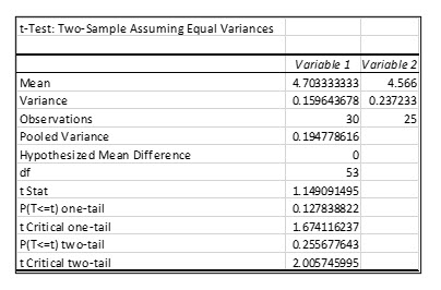
The result will display t statistics for both one and two tail tests. Excel also displays the critical values for each test in the output.

Two Sample Hypothesis Test – Proportions

Keisha is continuing her efforts to analyze and improve patient satisfaction. While patients interact with several nurses, Keisha realizes they seem to remember the nurse who discharged them, their last contact with the hospital, more than all the others. Keisha attempts to see if there is a difference in the overall patient satisfaction ratings between patients discharged by day shift nurses and those discharged by night shift nurses. Over the next week, Keisha randomly called several discharged patients and asked them if they were satisfied with the services offered at the hospital, allowing only “yes” or “no” as valid answers. Keisha uses patient records to see if they were discharged by day or night shift nurses.

Step 1: State the null and alternate hypothesis:

H0 Day shift nurse patient satisfaction = Night shift nurse patient satisfaction H1 Day shift nurse patient satisfaction <> Night shift nurse patient satisfaction

Step 2: Select the level of significance:

Keisha selects a .05 level of significance. This gives her a 5% chance of making a type I error.

Step 3: Determine the test statistic:

Because Keisha is working with proportions, she will use the z distribution.

Step 4: Determine the critical value (decision rule):

This is a two-tail test because Keisha is checking both directions, “different than”. With a .05 level of significance, each tail will have an area of 0.025. Finding the area of 0.475 in the normal distribution table, Keisha determines the critical value is 1.96.

Keisha surveys 55 discharged patients and finds that 25 were discharged by day shift nurses and 30 by night shift nurses. The results were as follows: Day shift discharge patients satisfied: 20/25 Night shift discharge patients satisfied: 25/30

The formula for computing a z score comparing two proportions has two steps.

The first step is to compute the pooled proportion.

The formula to do this is:

After computing the pooled proportion, you can then compute the z score with this formula:

The computed Z score is =.31884, falls within the “Do not reject” area because it is not greater than 1.96 or less than -1.96. Keisha will not reject the null hypothesis and conclude, based on this limited survey, the satisfaction ratings between patients discharged by day and evening nurses are equal.

Two Sample Hypothesis Test – Dependent Samples

The samples discussed and used in the examples so far are independent samples. That is, the patients surveyed about day nurses were not the same patients surveyed about night nurses. Other than being in the same hospital, there is no direct relationship between the two samples.

Conversely, a dependent sample is the same sample surveyed twice. The second survey is usually after an intervention such as a training, an adjustment, or a medication. The hypothesis revolves around the intervention and tests if the intervention resulted in a change, positive or negative. The same individuals are surveyed before and after the intervention.

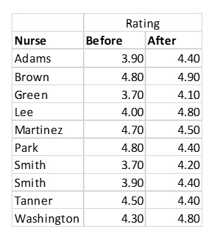
To illustrate a hypothesis test using dependent samples, assume Keisha decides to see if a training program can improve individual nurses’ patient satisfaction ratings. She decides to measure their mean ratings before and after the training. Keisha randomly selects ten nurses and records their patient satisfaction ratings for one week. After they attend customer service training, she records the same nurses’ ratings for the week after they complete training. Keisha is hopeful the training will improve patient satisfaction and sets out to test her hypothesis.

Step 1: State the null and alternate hypothesis:

H0 Ratings after training <= Ratings before training H1 Ratings after training > Ratings before training

Step 2: Select the level of significance:

Keisha selects a .05 level of significance. This gives her a 5% chance of making a Type I error.

Step 3: Determine the test statistic:

We will assume Keisha does not have the population standard deviation and therefore, she uses the t distribution.

Step 4: Determine the critical value (decision rule):

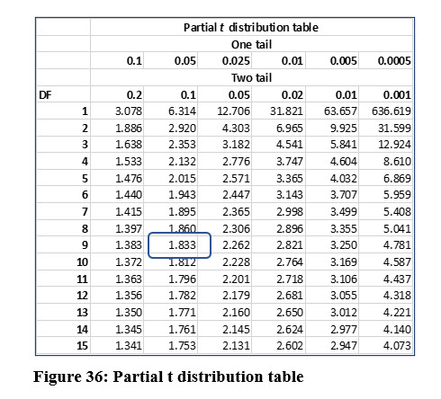
This is a one-tail test because Keisha is checking only one direction, “greater than”. The sample size is 10, even though the nurses were sampled twice. That means the degrees of freedom are 9. The critical value from the t distribution table in Figure 36 is 1.833.

Step 5: Take a sample, compute the test statistic and make a decision

Keisha gathers the ratings for the ten nurses before and after the training as shown below:

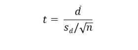
The formula to compute a t statistic from dependent (paired) samples is:

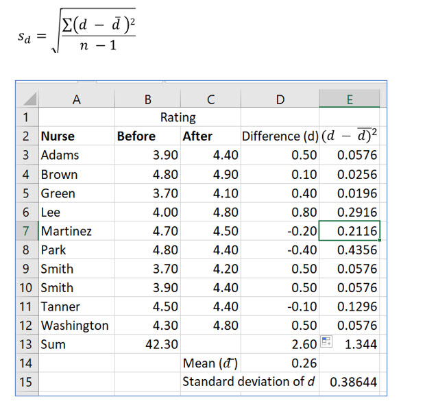
In this formula sd is the standard deviation of the differences between the before and after values. It is computed as:

Note that we compute the difference by subtracting the mean rating before then training from the mean after the training.

After computing the standard deviation of the differences, the t statistic is computed as:

The computed t stat is larger than the critical value of 1.833, so Keisha rejects the null hypothesis and concludes the training resulted in higher ratings for the nurses.

Try it in Excel:

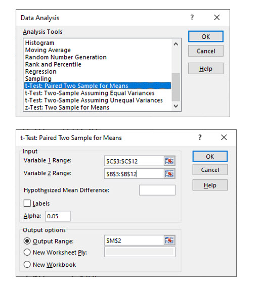
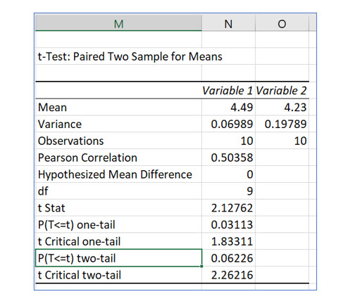
Excel’s data analysis add-in has a paired t test option that computes a t statistic for dependent samples.

To avoid computing a negative t statistic, the “after training” sample is Variable range 1.

As with the other t test options in Excel’s data analysis feature, the output table displays critical values for both one and two tail test as well as p values.

The p value for this one tail test is .03113. Keisha set up to test the hypothesis with a .05 level of significance. Keisha can also use the p value to determine whether or not to reject the null hypothesis. If the computed p value is smaller than the level of significance Keisha selected, she can reject the null hypothesis. If the p value is larger, she will not reject the null hypothesis.