Hypothesis Testing: One Sample

More Statistics Topics
Hypothesis Testing: One Sample

Hypothesis Testing: One Sample

This chapter in Surviving Statatistics explains how to complete a Hypothesis testing with one sample.

Instructional Videos

Surviving Statistics: Hypothesis Testing - One Sample Business Statistics: One Sample test of Hypothesis

Surviving Statistics Chapter 10 - File Downloads

Student Loan Debt

Hypothesis Testing: One Sample

You might recall from our first chapter that inferential statistics attempts to estimate, generalize, or predict something about a population. We introduced the concept of inferential statistics in the first few chapters. Then, we dug deeper into inferential statistics with the discussion of z scores and areas under the curve. Hypothesis testing is the formal process of checking the assumptions or inferences we have made. Researchers use hypothesis testing to test existing theories, propose new ones, test the effectiveness of a treatment or intervention, or just to compare two groups of observations. Hypothesis testing can also be used in quality control, such as checking the accuracy of weights and contents.

Hypothesis testing is a foundation of statistical research. From this point on, hypothesis testing will become an integral part of almost everything we do in this text with statistics.

Five Step Hypothesis Testing Procedure

Hypothesis testing can be a difficult concept to grasp. However, it really is not very difficult, especially if you follow the five-step hypothesis testing procedure in this chapter. This chapter will focus on hypothesis testing when we are comparing only one sample with a population.

Once you master the five-step process we introduce in this chapter, you will use it with many additional statistical computations. Several additional chapters of this text will rely on this same five-step procedure.

1. STATE THE NULL AND ALTERNATE HYPOTHESIS

Hypothesis testing requires two hypotheses, the null and the alternate. At the end of the hypothesis testing procedure, you will reject or not reject the null hypothesis. If you reject the null, then you may be able to accept the alternate. Here is an explanation of the null and alternate hypotheses:

The Null Hypothesis

The null hypothesis, H0, is what is assumed to be true, the status quo, “common knowledge,” or an established theory. In statistics, the null hypothesis is always expressed with some form of equality, such as <=, >=, or =.

For example, if a bag of potato chips states that it contains 8.7 ounces of chips, then the null hypothesis would be: chips in >= 8.7 ounces.

We include greater than 8.7 because to ensure there are no lawsuits, the production company will attempt to error on the side of too many chips, not too few.

The Alternate Hypothesis

The alternate hypothesis, H1 is mathematically contrary to the null hypothesis. Since the null hypothesis, H0, contains an equality, the alternate hypothesis will contain not equal to (< >), greater than (>), or less than (<).

Example #1:

Assume you oversee production at a potato chip company. Each bag is labeled that is has 8.7 ounces of chips. You need to constantly monitor the chip dispenser to ensure the bags contain at least 8.7 ounces of chips. Underfilling the bags would result in customer complaints and even, potentially, lawsuits. Because you think there may be a problem with the chip dispenser you develop the following hypotheses: Null, H0: Chip weight >= 8.7 ounces. Alternate, H1: Chip weight < 8.7 ounces. Note: You are only concerned about underfilling the bags with this example. In the “real world” over filling the bags would also be a problem. While overfilling the bags would make your customers happy, you may not stay in business very long by giving away your product. Without making this too complex, the solution businesses use is related to the confidence interval you learned about in chapter 9. You may, for example allow a margin of error of .1 ounces. Your chip dispenser might shoot for 8.8 ounces and is working properly (within tolerance) if it dispenses from 8.7 to 8.9 ounces.

Example #2:

You are testing a new procedure for making sandwiches at a fast food restaurant and believe your new method is faster and set out to test your theory. The null and alternate hypotheses would be stated as: H0: Mean assembly time with new procedure >= mean assembly time with old procedure H1: Mean assembly time with new procedure < mean assembly time with old procedure

Example #3:

You are testing the effectiveness of a new medication to treat a deadly virus. The null and alternate hypotheses would be: H0: Mean survival rate with new treatment <= Mean survival rate without new treatment H1: Mean survival rate with new treatment > Mean survival rate without new treatment

2. CHOOSE THE LEVEL OF SIGNIFICANCE

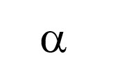
The level of significance, represented as , is the probability of rejecting a null hypothesis when it is actually true. To be considered statistically significant, levels of significance range from .1 to .01. Choosing a level of significance of .05 would mean you have only a 5% chance of rejecting a null hypothesis that is true, you are, therefore, 95% confident that you will not reject a null hypothesis that is true. Rejecting a null hypothesis when it is actually true is defined as a Type I error. The level of significance is the chance of making a Type I error.

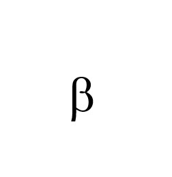
A type II error, represented by the symbol below occurs when you fail to reject a null hypothesis that is actually false.

3. DETERMINE THE TEST STATISTIC

Up to this point we have discussed the z statistic and the t statistic. When you are working with means, determining whether to use the z or t is dependent on the standard deviation. If you know the population standard deviation, you will use the z distribution. If not, you will use the t distribution. You will also use the z statistic when you are dealing with proportions.

You will learn additional test statistics in upcoming chapters. In the third step of the hypothesis testing procedure, you will choose which statistic to compute to make the decision to reject or not reject the null hypothesis.

4. LOCATE THE CRITICAL VALUE (DECISION RULE)

You will use the critical value to determine whether you do reject or do not reject the null hypothesis. The critical value is the test statistic value, z or t for now, that corresponds to the level of significance, (symbol below), you selected in step #2.

The critical value depends on whether you are doing a one-tail or a two-tail test, which you can easily determine by examining the null hypothesis.

One-tail tests examine the data in only one direction and have either <= or >= in the null hypothesis statement. Two-tail tests look at two directions and have = in the null hypothesis statement. 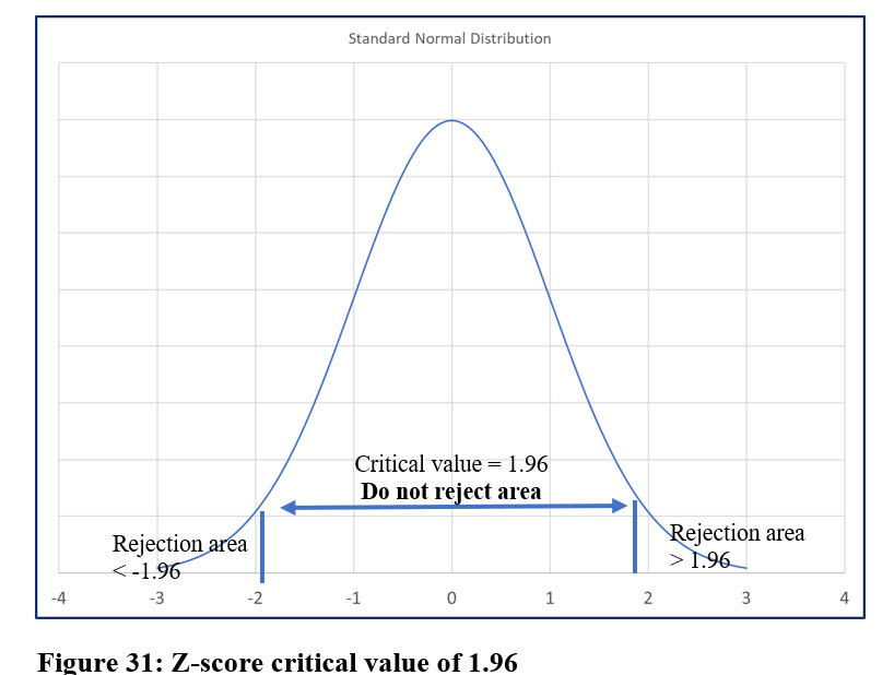One-tail test examples: Ho: Mean chips contents >= 8.7 ounces Ho: Mean survival rate with new treatment <= Mean survival rate without new treatment Two-tail test example: Ho: Sandwich assembly time new process = Sandwich assembly time old process We will delve into a complete example soon. In the meantime, here is a useful tip: if you are using a z statistic, with a two-tail test and a .05 level of significance, the critical z value is 1.96.

5. TAKE A SAMPLE, COMPUTE THE TEST STATISTIC AND MAKE A DECISION

In this final step of the hypothesis testing procedure, we will compute the test statistic. The formula depends on the test statistic and what you are comparing; one sample, two samples, a proportion, or something else.

After computing the test statistic value from your sample, compare it to the critical value you located in the previous step. The comparison of these two values determines whether you do or do not reject the null hypothesis.

You will reject the null hypothesis if the computed value falls within the rejection area, which will be in the tail or tails of the curve. If your computed has an absolute value greater than the critical value, you will reject the null. If the value you compute is smaller, do not reject the null hypothesis. Using our example two-tail null hypothesis and tip above: H0: Sandwich assembly time new process = Sandwich assembly time old process. Let’s say during the five-step hypothesis testing procedure, we set the level of significance at .05 and selected a z-test. Since this is a two-tail test, 1.96 is the critical value for z. Figure 31 shows the reject and do not reject areas based on a critical z-value value of 1.96. Do you reject the null hypothesis if the computed z-value is: a) 2.5? b) 1.0? c) -1.5? d) -2.5? Answer: a) Yes; b) No; c) No; d) Yes.

This process will make sense as we go through an example or two.

It also may be a good time to review Chapter 7 to ensure you understand z and t distribution curves and how to locate z and t scores before you delve into these examples.

One Sample Hypothesis Test – Known Population Standard Deviation

Dan’s Deli makes great sandwiches and is experiencing rapid growth. However, customers often complain about the wait after ordering before they receive their sandwiches.

Dan knows that right now it takes an average (mean) of 54 seconds to assemble a sandwich. In Dan’s past research, he learned the standard deviation of sandwich production is .7 seconds.

Marisol, one of Dan’s employees, has suggested some changes in the process including: rearranging some vegetable locations and changing the order of other ingredients. Marisol is sure her ideas will save time without sacrificing quality. Dan is quite skeptical but agrees to test her method to see if it saves time. Dan will test the method during the assembly of ten sandwiches and use the five-step hypothesis testing process to see if Marisol’s method is better or worse than the existing method.

Step 1: State the null and alternate hypothesis:

H0: µ = x̅ (The sandwich creation is the same, equal, for both methods.)

H1: µ < > x̅ (The sandwich creation time is not the same, not equal, for both methods.)

Step 2: Select the level of significance:

Dan selects a .1 level of significance. This gives him a 10% chance of making a Type I error, rejecting the null hypothesis when it is actually true.

Step 3: Determine the test statistic:

Since Dan has a population standard deviation from previous research on sandwich assembly, he will use the z statistic.

Step 4: Determine the critical value (decision rule):

This is a two-tailed test because Dan is pretty sure the assembly time will be the same, (i.e. equal) for both methods. However, the alternate hypothesis tests the time as either better or worse, (i.e. not equal).

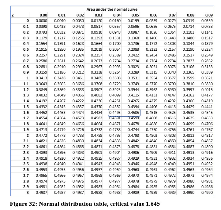
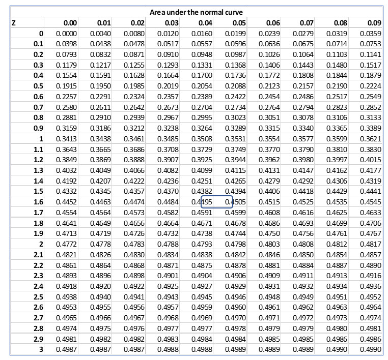
The critical z-value is determined from the following table in Figure 32. The level of significance determines the “do not reject” and “reject areas” under the normal curve. For two-tail, the area in each tail is 0.1 / 2 = .05 in each tail.

The “do not reject area” is 1 - .1 = .9 for both sides or .45 for each side in the area between the mean and each tail. The area .45 is not in the table. The closest areas are for z scores that equal 1.64 and 1.65. The area .45 is halfway between the listed areas of .4495 and .4505, so our critical value is 1.645, halfway between the two listed z scores.

From this, the takeaway is: The critical value is: 1.645 .1 level of significance .05 in each tail .45 area between mean and tail.

Step 5: Take a sample, compute the test statistic and make a decision

The mean assembly time for the sample of ten sandwiches was 53 seconds using Marisol’s revised process.

The formula to compute a z score from one sample mean is:

Because the computed z score, -4.512 falls outside -1.645 and 1.645 and is the reject area. Dan is forced to reject the null hypothesis. He concludes, at the .1 level of significance, there is a statistically significant difference between the old and Marisol’s proposed assembly methods. Based on the test results, Dan promotes Marisol and encourages her to look for even more ways to increase efficiency.

One Sample Hypothesis Test – Unknown Population Standard Deviation

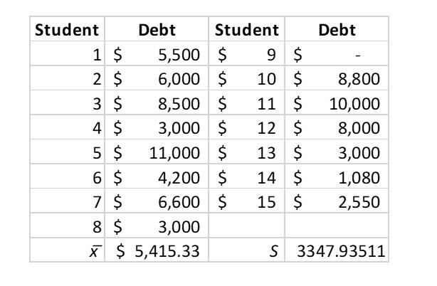
Cindy, an astute high school senior, is considering a nearby private college which advertises is generosity in awarding scholarships and grants. On its website, it states students graduate with and average student loan debt of only $5,000. Cindy believes this number is too low and devises a plan to test her hypothesis. She surveys 15 college seniors a month from graduation.

Step 1: State the null and alternate hypothesis:

H0: µ <= $5,000 (The average student loan debt is less than or equal to $5,000.) H1: µ > $5,000 (The average student loan debt is greater than $5,000.)

Step 2: Select the level of significance:

Cindy selects a .05 level of significance. This gives her a 5% chance of rejecting the null hypothesis when it is actually true, a Type I error.

Step 3: Determine the test statistic:

The college only posted the mean, not the standard deviation. Since Cindy does not have the population standard deviation, she will use the t statistic.

Step 4: Determine the critical value (decision rule):

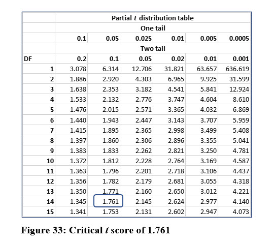
This is a one-tail test because Cindy is only checking one direction. To find the critical value, the t statistic uses degrees of freedom which, with only one sample, equals one less than sample size, n – 1. With a sample size of 15, the degrees of freedom are 14.

As illustrated in Figure 33, using the .05 level of significance for one tail column with 14 degrees of freedom, the critical t statistic is 1.761.

Step 5: Take a sample, compute the test statistic and make a decision:

Cindy’s survey found the following:

The formula to compute a t score from one sample mean is:

Because the computed t score, .48046, is less than 1.791, Cindy does not reject the null hypothesis . She cannot conclude, at the .05 level of significance, that the mean student loan debt is greater than $5,000.

Note: Cindy computed a sample mean that is higher than the population mean reported by the college. Why can she not reject the null hypothesis and conclude the school is guilty of false advertising?

Because the .05 level of significance only tolerates a 5% chance that an actually true null hypotheses is rejected in error. The bottom line is that Cindy’s chances of making a Type I error are greater than what the testing procedure she established will accept. Her chances of making a Type I error are far greater than she specified when she began the test. In fact, the probability (p value) of making a type I error with a t statistic of .48046 and 14 degrees of freedom is 34.47%.

Excel’s T.Dist() function computes the p value from a t statistic.

What does Cindy need to do to prove that the college is guilty of false advertising? She needs to increase her sample size (i.e., the number of students in her survey)! This makes sense because a survey of fifteen students is really too small to accuse the college of false advertising.

Hypothesis Test – One Proportion

A recent study that found that 33% of college students change majors in the first three years of college. Mario does not believe that the percentage is this high at the college he attends. He devises a plan to test his hypothesis, which involves randomly surveying fifty seniors at the college he attends.

Step 1: State the null and alternate hypothesis:

H0 The proportion of seniors who changed majors is >= 33/100 H1 The proportion of seniors who changed majors is < 33/100

Step 2: Select the level of significance:

Mario selects a .05 level of significance which gives him a 5% chance of making a Type I error.

Step 3: Determine the test statistic:

Because Mario is working with proportions, he will use the z statistic.

Step 4: Determine the critical value (decision rule):

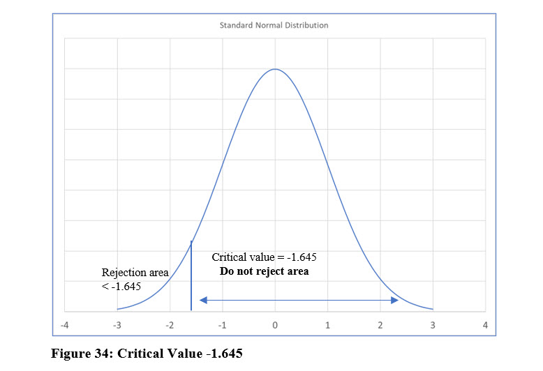
This is a one-tail test because Mario is only checking one direction, < 33%. The z score for an area of .45 (5% in the single tail) equals 1.645 because .45 is halfway between the two areas for the z scores of 1.64 and 1.65. Because the rejection area, the tail, is on the left side of the curve, the critical value is actually -1.645 as shown in Figure 34. Remember Mario thinks the percentage is less than 33%.

Step 5: Take a sample, compute the test statistic and make a decision:

Of the fifty seniors Mario surveyed, ten reported changing majors in their first three years.

The formula to compute a z score from one proportion is:

Mario computed a z score which is more negative than the critical value. He will reject the null hypothesis and conclude, that at least at his school, the reported proportion may not be correct.