Printing & Page Setup Features
Easy to follow step-by-step instructions and videos help you learn to use Excel's printing and Page Setup features including scaling and printing a portion of a worksheet, adding gridlines, changing the orientation, and adding headers and footers.
Note: These instructions are excerpted from Luther Maddy’s Excel Workbooks (C) 2024 which are available in printed or eBook format from Amazon.com
Watch the video-Printing tips and tricks
Download Excel Printing Features Exercise File
Printing Features
Printing is a very easy feature. Because worksheets may be quite large, most of the time you may not want to print the entire worksheet. In this lesson you will learn how to specify only certain parts of the worksheet for printing. You will also learn to add features such as headers and footers.
1. Open the No Fault Travel workbook.
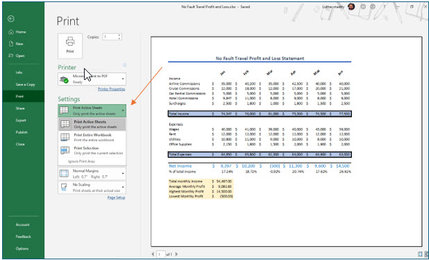
2. Open the File menu and choose Print.
Printing a Worksheet
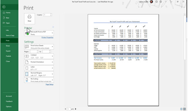
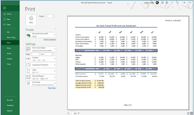
Choosing the Print command box allows you to select certain portions of the worksheet and even which pages to print. You can also see a preview of the printed worksheet. Clicking the Print tool on the toolbar automatically prints the entire worksheet. The other options in this menu include letting you specify what portions of the worksheet you would like to print, how many copies to print, and what printer to use when printing.
Notice that the print preview shows the data that will not fit on the first page. As it is now, this worksheet takes two pages to print. You can verify this by examining the page indicator near the bottom center of the screen.
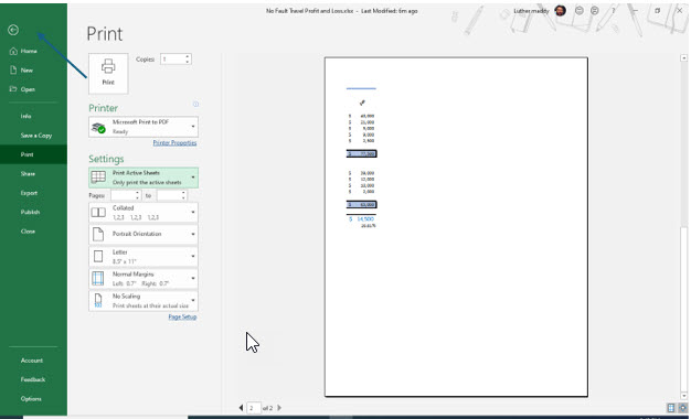
3. Click the Next Page arrow at the bottom of the print preview area.
You now see the information that would print on the second page.
4. After viewing the Print Preview, click the Back arrow at the top left of the File menu to return to the worksheet.
Adjusting Print Options
If you want this entire spreadsheet to fit on one page you can shrink the font and column widths on the worksheet. Or, you could tell Excel to shrink the information to have it fit on one page. You could also change the page orientation to Landscape. We’ll first have you tell Excel to fit this all on one portrait page.
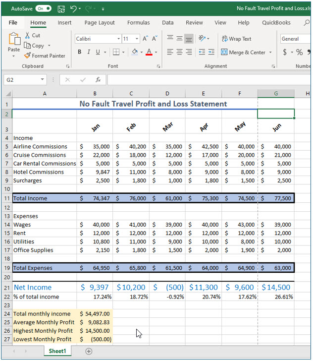
Returning to the worksheet you should notice that Excel has added a dotted vertical line on your worksheet between columns F and G. This line represents a page break. From your screen, or the image below, you should clearly see that column G will not print on the first page of the worksheet.
You will now inform Excel that you want to fit the worksheet on just one page.
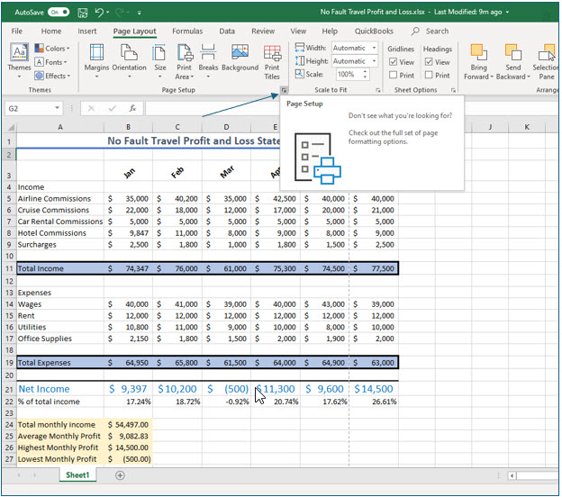
1. Click the dialog box launcher on the Page Setup group on the Page Layout tab.
You can click the launcher from either the Page Setup, Scale to Fit, or Sheet Options group in the Page Setup on the ribbon.
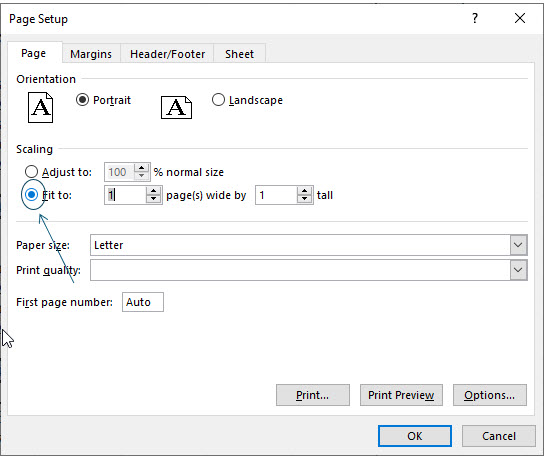
You should now see the Page Setup dialog box. Many of the options available here are also available on the Ribbon.
2. If needed, click the Page tab in the Page Setup dialog box. Next, click the Fit to radio button and ensure the options are 1 page wide by 1 page tall.
You have now given Excel the command to shrink all the data in this worksheet to fit on one page during the printing process.
3. Click OK to leave this dialog box.
You should notice the page break between column F and G is gone. You could have also changed this setting by using the ribbon. In the Scale to Fit group you should now see that the width is set as 1 page, as is the height. You can change this setting by using the drop-down arrow for each of these tools.
4. Click File to open the File menu and choose Print.
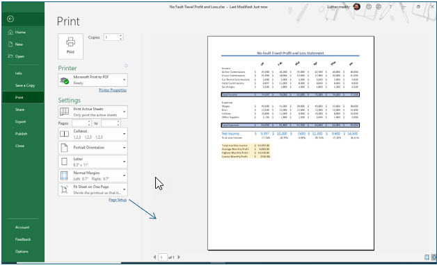
You should see that the entire worksheet is displayed and will fit on one page.
Printing a Partial Worksheet
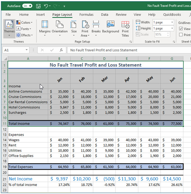
As you have just seen, Excel prints the entire worksheet unless you tell it otherwise. If you do not wish to print the entire worksheet, first select the cells you want to print. Then, open the File menu, but before selecting print you will choose Print Selection in the settings section. In this portion of the lesson, you will specify that only a portion of the worksheet prints.
1. Return to the worksheet and then select cells A1 through G11.
2. Click File, then choose Print.
Notice that according to the Print Preview section, the entire worksheet will be printed. You need to inform Excel that you only want to print the cells you have selected.
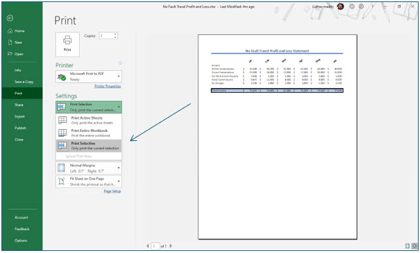
3. In the Settings section, choose Print Selection.
After selecting this option, as you examine the preview, you should notice that only the selected cells are displayed. If you had chosen to print to a printer, the result on paper would be the same.
5. Return to the worksheet by clicking the left arrow at the top left instead of actually printing.
For this lesson, you will save paper and ink as you explore Excel’s printing features by not actually printing the worksheet.
Changing the Orientation
By default, Excel chooses to print this worksheet information in portrait orientation. Turning the page sideways (landscape) allows you to print more columns. In this portion of the lesson you will change the orientation to landscape and observe the changes.
1. In the Scale to Fit group, change the width and height back to Automatic by clicking the drop-down arrow in each section.
As you changed the width and height options, you should notice that Excel now displays where the page break again between columns F and G.
You will now change the orientation to landscape. This will allow more columns to fit across the page when the worksheet is printed.
2. In the Page Setup tab, click the Orientation tool and choose Landscape.
When you returned to the worksheet, notice that Excel has moved the page break over a couple of rows. This reflects the change in orientation to landscape.
You can also change the orientation and several other options by going into the Page Setup dialog box or even when after you have selected the Print command. There is no one “right way” to select Excel commands.
4. Click File and choose Print.
Notice the preview section shows the orientation change.
5. Change the Print Settings back to Print Active Sheet from Print Selection.
As you view print options you should notice that Landscape orientation is selected. You could have also changed the orientation here without having to return to the worksheet.
Adding Headers and Footers
As you examined the print preview you may have noticed the absence of page numbers. By default, Excel does not add page numbers and other information at the top or bottom of the page. In this portion of the lesson you will add header and footer information, including page numbers to the printout.
1. Close the Print menu and return to the worksheet. Then, click the Page Setup dialog box launcher again.
There are many pre-defined headers and footers which in most cases will give you the exact options you need. However, we’ll have you create headers and footers from scratch so you can learn more about their use.
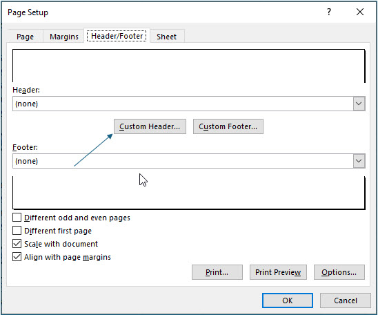
2. In the Page Setup dialog box, click the Header/Footer tab then click the Custom Header button.
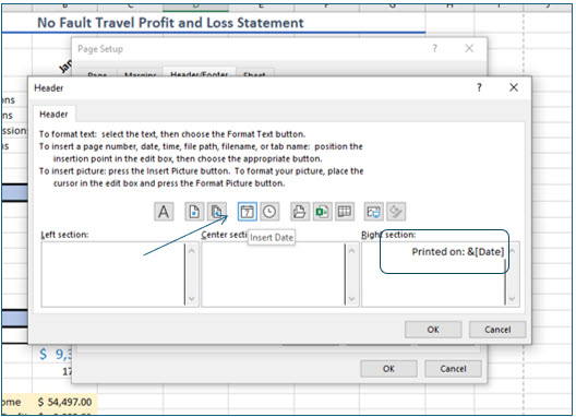
You should now see the Header dialog box which consists of three sections: left, right, and center. There are tools in this dialog box to insert Excel generated items in the header like the page number, file name, and current date. You can also type custom text in any of the three sections.
3. Press (Tab) twice to move to the Right section of the header.
4. In the Right section of the header type Printed on: and then insert a (Space).
5. Click the Insert Date tool in the Header dialog box.
You should now see &[Date] in the right section. When you print, Excel will add the current date. You should use the Date code rather than typing the date so that the date on the printout will let you know exactly how current the spreadsheet printout is.
In addition to creating a custom header or footer as you just did, Excel has several pre-created headers and footers you may be able to use. In this portion of the exercise you will use a pre-created footer.
6. Click OK to return to the Header/Footer tab.
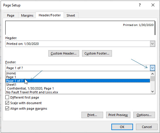
7. Click the Footer drop-down list button, choose Page 1 of ? and then click OK.
The header and footers you just added to your worksheet will not display on the worksheet. They will appear when you print the worksheet or view it in Print Preview.
8. Click File and then choose Print.
9. In the Print menu, change the Settings to print Active sheets instead of Selection.
You should see the header and footer in the print preview.
The Page Layout View
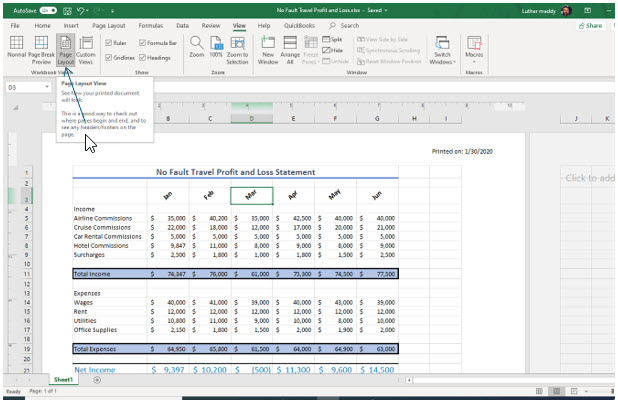
If you want to see options normally not visible in the editing mode, like headers and footers, you can change the view to the Page Layout view. In this mode you can work with your worksheet as well as see headers, footers, and a better representation of page breaks.
1. Return to the worksheet from the Print menu and then click the View tab.
2. In the View tab, click the Page Layout tool in the Workbook Views group.
You should now see the header and footer you just created.
The Page Layout view allows you to work with the worksheet as does the Normal view. The difference is that you can see page formatting options.
3. In the View tab, click the Normal tool in the Workbook Views group.
Excel has now returned to the Normal view.
Printing Gridlines
As you examined the print preview, you may have noticed that the only lines that appear are the ones you added to the worksheet. It is possible to have Excel print gridlines around each cell. With gridlines added, the printout will resemble the layout of the actual worksheet as you work with it. You can add gridlines from Page Setup.
1. Click the Page Layout tab and launch the Page Setup dialog box.
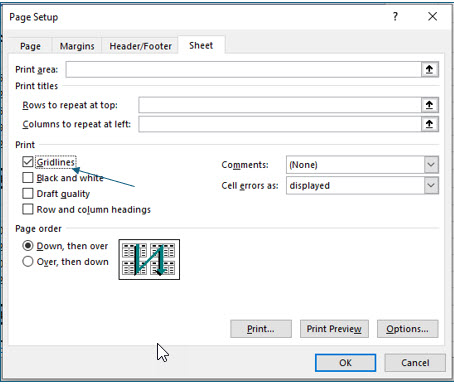
2. In the Page Setup dialog box, click the Sheet tab.
3. In the Sheet tab, click the Gridlines check box and click OK.
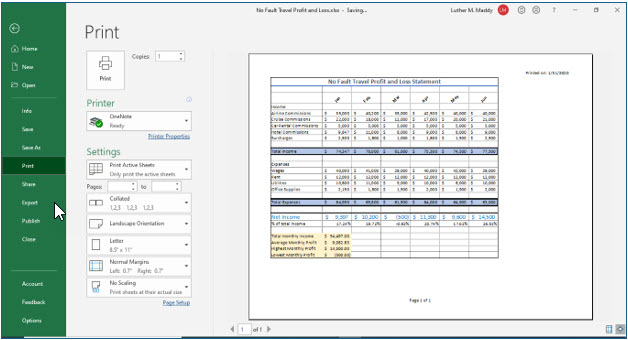
4. Click the File tab again and choose Print.
You should now see that Excel added cell gridlines to the print preview.
5. Save and close the No Fault Travel P&L workbook.
