Working with Multiple Worksheets
This lesson includes step-by-step instructions to teach you to create and use multiple worksheets in a workbook and link them using three-dimensional formulas.
Note: These instructions are excerpted from Luther Maddy’s Excel Workbooks (C) 2024 which are available in printed or eBook format from Amazon.com
Watch the video-Working with Multiple Worksheets
Download TripData to complete the lesson
Working with Multiple Worksheets
When you open a blank workbook in Excel, you are provided one worksheet, but you can add additional worksheets, which are basically additional “pages” in the workbook. Separate worksheets are useful for organizing different categories such as different departments, vendors, or customers. Multiple worksheets are especially useful for computing the same values for several time periods, such as months, days, or years. In this lesson, you will use multiple worksheets to track No Fault Travel trip sales values for three different months.
1. Open the No Fault Travel Sales Report workbook you created in the review lesson. Use the Save as command and save this as No Fault Travel Summary Report.
If you have the Excel’s auto save feature turned on, it will save the workbook every time you make a change. In this case, you want to original to remain as it is, so you are creating a copy with a new name before you make any modifications. If you did not create this copy and have Auto Save turned on, you will lose the original workbook as Excel will automatically replace it with the modifications you are about to make.
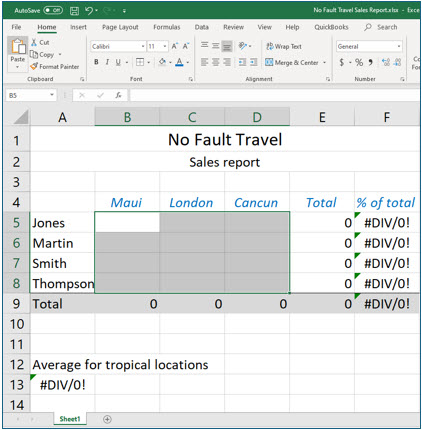
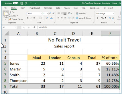
2. Select cells B5 through D8 and press the (Delete) key to erase the current values.
YMake sure that the cells you select only encompass the sales data and not your formulas you placed in column E and F or row 9. Leaving the formulas intact will save you time and effort.
You are going to use this worksheet without data as a template to use several places. The data will be different, but the formulas will remain the same throughout.
3. Save your work again and ensure it is called No Fault Travel Summary Report.
If you have the Auto Save feature on, Excel saves for you.
Inserting Worksheets
Each new Excel workbook has only one worksheet. However, you can add additional sheets, if you need them. When you insert a new worksheet, Excel will place the new sheet after the last existing worksheet.
1. Click the Insert Worksheet icon.
You should now see that Excel created a new worksheet after Sheet1. It named this worksheet Sheet2 because it is the second sheet added to the Workbook. After Excel created this new worksheet, it made that worksheet active. You can move from sheet to sheet by clicking on its sheet tab.
2. Click the Insert Worksheet two more times.
You should now have four worksheets to work with.
Renaming sheets
If you are using several worksheets in a workbook, referring to them by their default name (Sheet1, etc..) may cause confusion and you may even forget what sheet stores what information. Fortunately, you can easily rename the worksheets in a workbook. Renaming worksheets helps you or anyone else who may use this workbook understand what each worksheet refers to. It also makes creating formulas based on values from other worksheets easier too.
One of the easiest ways to rename a worksheet is to simply double-click on its tab. This will select the existing name and you can then type the new name. You can also rename a worksheet by accessing the sheet’s shortcut menu by right-clicking on its tab.
1. Double-click on the tab for Sheet1. When Sheet1 is selected, type Jan and press (Enter).
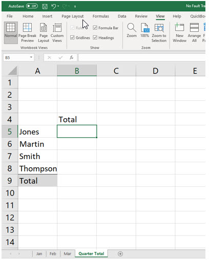
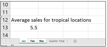
2. Use the same method to rename the remaining sheets Feb, Mar and Quarter Total as shown below.
Copying information between worksheets
The January worksheet has the template with the formulas already created. All you need to do on this worksheet is enter the month’s data and the totals, percentages, and average will be computed using the formulas you already created.
You will also be able to use this same template for the February and March worksheets. So, rather than entering all the information manually for each of these additional worksheets, you will just copy the template from the January worksheet to the February and March worksheets. When you do copy from one sheet to another, the formulas will adjust to the new worksheet.
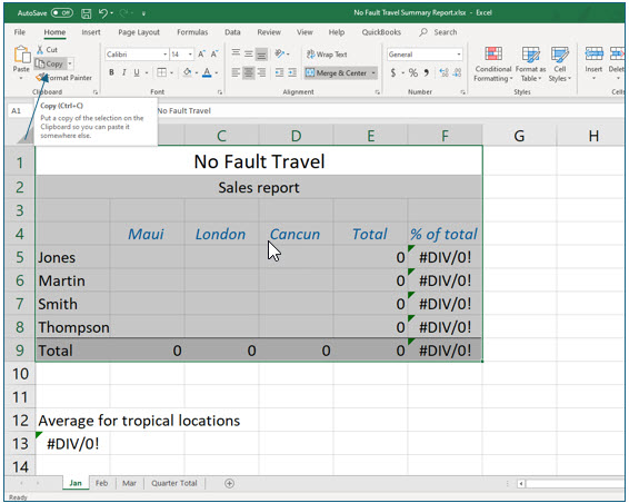
1. Click the January worksheet tab to make it active. Then, select cells A1:F9 and then choose the Copy command.
You have now placed the data and the formulas from the cells you copied into the clipboard. You will paste this information into the other worksheets that need this template. This selection does not include the average information. You will not copy that information at this time, although you certainly could and it would work properly on the new sheet.
2. Switch to the Feb sheet, make sure A1 is the active cell and then execute the Paste command.
You pasted beginning at cell A1 so that the cell addresses will be consistent from one sheet to another.
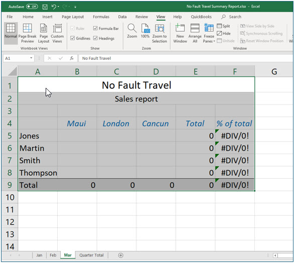
3. Move to cell A1 in the Mar sheet and paste again.
You should have a copy of the template in the Jan, Feb and Mar worksheets. You did not paste this information into the Quarter Total sheet because it will contain different information than the other three worksheets.
The cells you copied in the January worksheet will still be selected. You will also see the dashed marquee around the cells you copied. You can remove this marquee by pressing the (Esc) key or just by entering new data.
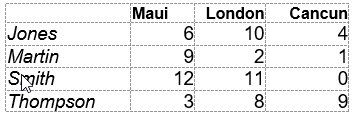
4. Move to the Jan sheet and enter the values shown below.
The total and % of total cells will be computed for you as you are entering these values because you left the formulas when you erased the data.
5. Enter the values below into the Feb worksheet.
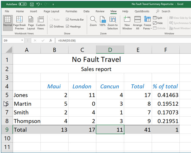
6. Enter the values below into the Mar worksheet.
You now have values in the worksheets for all three months. You will now create formulas in the Quarter Total worksheet that add the values from all three months.
7. Copy cells A5:A9 from the Jan worksheet and paste the copy beginning at cell A5 in the Quarter Total sheet.
8. In cell B4 of the Quarter Total worksheet type Total and then move to cell B5.
Linking worksheets
The Quarter Total worksheet will display the total of all three months for each salesperson. You will do this by creating a formula. This formula will be linked to the other worksheets. Because these formulas will be linked to the values in other worksheets, the results of these formulas will change if the values in the other worksheets should change.
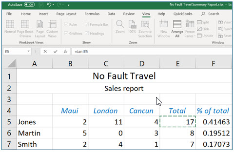
To create a formula that refers to a cell on another worksheet you can either type the formula or you can use the “point and click” method. Regardless of the method you use the syntax is the same. The syntax for a formula that refers to a cell on a different worksheet is: =Sheetname!cellAddress. In other words to create a formula that refers to cell E5 on the Jan worksheet, the formula would be: =Jan!E5.
When you create linking formulas manually, you have to remember to separate the sheet name and the cell address with an exclamation point (!). You also need to ensure that you spell each sheet name exactly in the formula. Using the “point and click” method to enter formulas eliminates some of the potential for error because Excel does the typing instead of you. This lesson will step you through using the “point and click” method to create a formula that adds the totals of all three months on the Quarter Total worksheet.
1. Move to the Quarter Total worksheet and in cell B5, begin a formula by pressing the (=) key.
This formula will sum all the sales for Jones. Instead of typing the cell addresses, you will use the “point and click” method.
2. Click on the Jan worksheet tab and then click on cell E5.
You should notice that the formula bar displays the sheet name and the cell address. .
3. Type a (+) and then click on the Feb worksheet tab.
The name of this tab should also be added to the formula you are creating.
4. Click on cell E5 in the Feb tab and then type another (+).
You will now complete the formula by adding the March total for Jones.
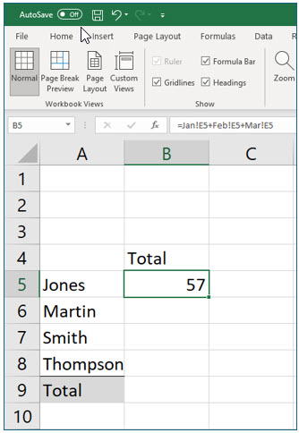
5. Click on the Mar tab, click on cell E5 and then press (Enter).
The result of the formula appears in cell B5. If you move back into cell B5 you should now see the completed formula in the formula bar. If your formula does not appear as it should, move back into cell B5 and try creating the formula again. Some of the most common errors users make when creating these formulas is forgetting to click on the cell after selecting the worksheet and adding a plus (+) after clicking on the last cell rather than pressing the (Enter) key.
Using Functions when Linking worksheets
Excel provides functions to make creating complex formulas easier. Rather than creating a formula that refers to each sheet and cell individually, as long as you are referencing the same in each worksheet, you can use the Sum function to build the formula. Doing so you would create the formula as: =Sum(Jan:Mar!E5). This would be a more practical approach for adding the values in several worksheets. Typing this formula works fine if you have the sheet names typed properly. You could also use other functions when linking worksheets such as Average, Count, Min, and Max.
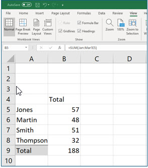
1. Replace the formula in Cell B5 of the Quarter total worksheet with =Sum(Jan:Mar!E5). Then, use the fill handle to copy the formula from B5 to B6:B9.
If you have difficulty with this formula, you can use the original version. If you see #REF! in the call, you have misspelled a sheet name. A common error is adding a space when naming the worksheets. If this is the case, you can correct this by renaming the sheets correctly, without a space.
This is a “copyable” formula. The cell addresses are relative and adjust as they should when you copy the formula. Sheet names are absolute and do not change when you copy the formula, which is exactly what you want when copying this formula on the same worksheet.
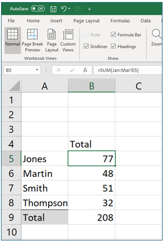
2. Move to the Jan worksheet and change the Maui value, cell B5, for Jones from 2 to 22.
3. Move to the Quarter Total worksheet and verify that it now reflects the changed value.
4. Save the worksheet.
This workbook is not yet complete but saving at this point reminds you to practice periodically saving your work. Save early and often and avoid recreating your worksheets.
Grouping Worksheets
There may be times when you want to do the same thing in all, or several, worksheets. For example, maybe you would like to italicize some cells or change the color of other cells in multiple worksheets. If you had formatted the January worksheet exactly as you wanted all the others to appear before you copied the data, those worksheets would have the same formatting. Now, however, if you change formatting on one worksheet, you will have to repeat the process on every other worksheet individually, unless you use the grouping feature.
Without the grouping feature you would have to enhance those cells in each worksheet, one at a time. By grouping the worksheets, you can change the formatting of one worksheet and have all the other sheets get the same formatting changes. Changing formatting options works well with the grouping feature, but only when the grouped worksheets have the same information in the same cells, as the Summary Report workbook does.
Grouping worksheets is very easy. You can group worksheets by clicking on the first worksheet tab and then, while holding down the (Shift) key, click on the last worksheet to be included in the group. If the worksheets are not contiguous (together), you can use the Control+Click method to select multiple non-adjacent worksheets.
1. Click on the Jan worksheet tab. Press and hold the (Shift) key and then click the Mar tab.
You notice that all three sheet tabs are now selected. While the worksheets are grouped, whatever you do to one worksheet will be done to all. That includes changing values and formulas, so be very careful what changes you make when you have multiple worksheets selected.
2. Select cells B4:F4, the titles in Row 4.
Even though you cannot see it, Excel has selected these cells in all three worksheets.
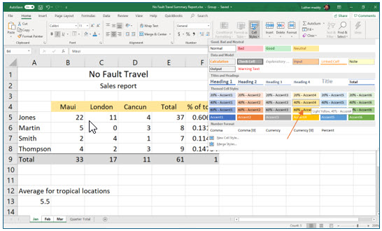
3. Click the Cell Styles tool on the Home tab and then select Light Yellow 40% Accent4.
If you click on the sheet tabs for Feb and Mar you will see that the titles in each worksheet now have the same cell style.
4. With the sheets still grouped, change the formatting in Cells F5 through F9 to percentage with two decimal places.
Ungrouping sheets
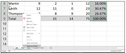
When you no longer need the worksheets to be grouped, you should be careful to un-group them. If not, you could accidentally change data in several worksheets. To ungroup worksheets you can simply click on a sheet that is not part of the group. In the event that all sheets are grouped, you can right-click any sheet tab and choose Ungroup Sheets from the shortcut menu.
1. Right-click the Feb worksheet tab.
You should now see the Worksheet shortcut menu.
2. Choose Ungroup Sheets from the shortcut menu.
You should notice that none of the sheets are grouped.
Changing tab colors
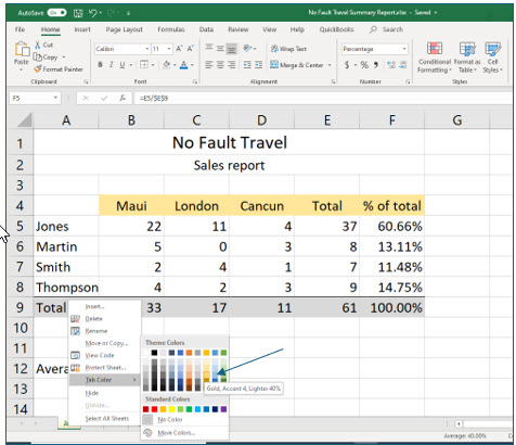
In addition to renaming worksheets, you can also change their colors. This makes them easier to identify when you are working with several worksheets. To change the color of a sheet tab, you can right-click any sheet tab and choose Tab Color from the shortcut menu.
1. Right-click the Jan worksheet and choose Tab Color.
You should now see the available colors for sheet tabs. You can also choose the More Colors… option to choose from an even larger list of tab colors.
2. Choose Gold, Accent 4, Lighter 40% for the January tab.
The color you choose is not all that important for this lesson. You can choose different colors if you like. After choosing a tab color, you will not see the color change until you select another worksheet tab.
3. Change the tab colors for the remaining worksheets to any colors you desire.
4. Save the workbook after making these changes and then Close it.
Saving the workbook with the Save or Save as commands saves all the worksheets, not just the one that is currently selected.
