Moving & Copying Data and Formulas

More Excel Topics
Moving & Copying Data and Formulas

Moving & Copying Data and Formulas

These step-by-step instructions will help you learn how to copy and move both data and formulas in Excel. You will learn when a formula can be copied without modification and when you will need to modify a formula before copying it.

Watch the video-What's the best way to move and copy in Excel?

Download Excel Moving and Copying Excercise File

Moving & Copying Data and Formulas

Excel is a very flexible program. You can easily edit cell contents and move and copy data and values. In this lesson, you will rearrange the spreadsheet by moving and copying. You will also learn about copying formulas and when a formula can be correctly copied and when it cannot.

Opening an Existing Workbook

After closing a workbook, you will need to open it to continue working on it. You’ll now open the No Fault Travel Profit and Loss file you created in Lesson #1, to use in this portion of Lesson #2.

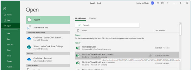
1. Click File and then choose the Open command.

Excel will now list all the Workbook files you have worked on recently. If the file you need is not here you can click the Browse tool and navigate to the correct folder.

2. Click No Fault Travel Profit and Loss in the list of Recent Workbooks to open this file.

You should now see the No Fault Travel P&L workbook just as you left it when you closed it. Excel even remembers which cell was active when you last saved the file. When you open the workbook file, you will notice the active cell may not always be cell A1. The key combination, (Control+Home) will quickly move to cell A1.

Editing Cell Contents

Excel provides several ways of changing or editing cell contents. To replace the entire entry of a cell you can just type over the value you do not want. To change just a portion of a cell’s contents you can edit the cell’s contents instead of replacing it. To edit a cell’s contents move into that cell. Then, click in the Formula bar (Active cell contents) and make the necessary changes.

1. Move to cell C8, the value for Hotel Commissions type 9847, then press (Enter).

You replaced the old contents with the new value. Notice also that the total income and net income also changed automatically to reflect the new value. This is because you created the formulas using cell addresses.

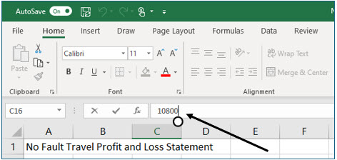
2. Move to cell C16, the value for Utilities.

This time you will leave most of the existing contents intact and simply edit this value instead of replacing it.

3. Click at the end of this cell’s contents in the Formula bar.

4. After you see the insertion point (cursor) blinking at the end of the current value, type a 0 to change the value to 10800 and then press (Enter).

As it did before, Excel will update all the formulas to reflect this change.

Selecting Cells

Before you can move or copy cells, you must first select those cells. By selecting cells, you inform Excel which cells you wish to move or copy. You will also need to select cells for many other operations, such as format changes.

There are several ways to select cells. The most basic is to click and drag. However, to select cells, start in the middle of that cell. When you are in the correct place for selecting cells, the mouse pointer will resemble a white plus symbol ( ).

Should you wish to select an entire column or row, you can click on the column or row heading to select every cell in that row or column. Should you wish to select more than one entire column, you can do so by clicking and dragging to select multiple column or row headings.

In addition to using the mouse, you can also select cells with the keyboard. To do this, move to the first cell you wish to select. Then, press and hold the (Shift) key and then press an arrow key in the direction you want to select. As long as the (Shift) key is depressed, any movement command will highlight cells.

Selecting non-contiguous ranges

Sometimes you may need to select groups of cells that are not together. To select non-contiguous groups of cells, select the first group of cells with the mouse. Then, press and hold the (Control) key and then select the second group of cells. As long as you hold down the (Control) key, you can select as many separate ranges as you wish.

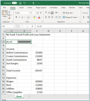
1. Move to cell A3.

2. Ensure that the mouse pointer resembles a white plus ( ) and then click and drag to cell B3.

You should notice that the cell you started with is not shaded. However, the thick black border tells you that both cells are selected. Excel leaves the starting cell white so you know where you started selecting cells.

3. Press (Delete) to delete the contents of the selected cells.

You have now deleted the date and the date label. The (Delete) key will delete the contents of all selected cells. If only one cell is active, it will delete that one cell’s contents. Remember the ####’s in the cell indicate the column must be wider to display that cell’s contents.

4. Move to cell C11 and press (Delete).

As you saw earlier, the AutoSum formula was a better approach to adding a column of numbers than entering the formula that contained a reference to each cell to be added. You will now replace the formula you created by using the AutoSum feature.

5. Click the AutoSum tool on the Home tab and then press (Enter).

The amount in the calculated cell will be the same as before, however, this formula is much better in the long run as you will see in future lessons. If you move into this cell and view the formula, you will see that it sums adds C6 through C10. The colon (:) represents “through”. This means, as you will see later, if you insert additional rows between C6 and C10, the values you enter will be included in the total.

Moving Cells

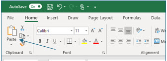
To move cells from one location to another the first step is to select the cells you want to move. After selecting those cells, you then choose the Cut command. After choosing the Cut command, move where you want the new cells to appear. After moving to the new destination, choose the Paste command.

One thing that can make the moving and copying process somewhat complex is the several methods available for accessing the Cut, Copy and Paste commands. For example you can find these commands the following ways: On the Home tab in the clipboard group. Right-clicking on selected cells. Keyboard shortcut keys: (Control+x) = Cut, (Control+c) = Copy, & (Control+v) = Paste

There is no right or wrong way to select a command. Most commands in Excel can be executed multiple ways. The best method of selecting a command is the one you remember. However, after you become more comfortable with Excel, you’ll probably want to become more efficient at it. Then, learning more than one way of performing an operation will save time.

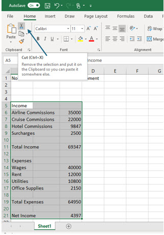
1. Use the click and drag method to select cells A5:C21.

Excel uses (:) to represent “through”. Remember that to select cells the mouse pointer must resemble the white plus symbol.

2. With these cells selected, click the Cut tool on the ribbon on the Home tab.

Unlike other programs you may use, the selected cells do not disappear when you choose the Cut command. Instead, Excel places a marquee around the cells so you know which ones will move. The process will not be complete until you actually choose the Paste command. You may have also noticed that when you pointed to the Cut tool Excel display more information about that command, including the keyboard shortcut, (Control+X), that you could have also used.

3. Click in cell A4 and then click the Paste tool on the Home tab.

The Paste tool has a drop down arrow, but you do not need to use that now. Clicking the tool icon will cause Excel to paste the cells you cut, beginning at cell A4.

All of the selected cells will now move up one row. As discussed earlier, you could have also accessed the Cut and Paste command using any of the additional methods Excel provides with the same results.

The cells you moved contained three cells with formulas. As you moved these cells, Excel automatically adjusted the formulas to fit their new location. For example, the formula that computed the new income was =C11-C19. If you examine this cell now, you will see that Excel adjusted the formula to become =C10-C18. This is one of the most powerful features of Excel. When you move, insert, or delete cells, Excel will automatically adjust the formulas in the worksheet.

Using the Fill Handle

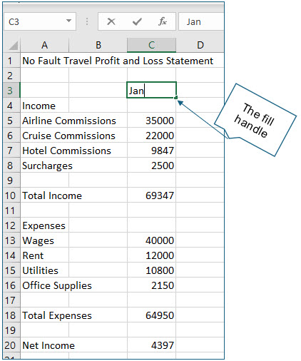
The fill handle (the skinny black plus at the right edge of the active cell) provides a very quick way to copy a cell’s contents. It is particularly useful for copying formulas.

Another feature of the fill handle is that it will attempt to increment text values such as months or days of the week. This is very useful if you are creating column headings representing several consecutive months. You’ll use the fill handle now to create headings for additional months of the year. You’ll also use it to copy formulas.

1. Move to cell C3 and type Jan.

It’s not necessary to press (Enter) after typing Jan. If you do, you’ll need to move back into cell C3.

2. Locate the fill handle at the bottom right corner of cell C3.

When you are in the correct location, the mouse pointer will resemble a small black plus symbol.

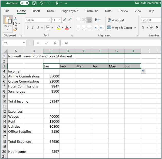
3. Click and drag the fill handle to cell H3 and then release the mouse.

Excel will then fill the cells you selected, incrementing month names. If cell C3 had contained January, Excel would have incremented the other cells with the full month names as well. The fill handle increments month names, days of the week, and numeric patterns.

Copying Formulas

One of the most common things to copy in Excel are formulas. For example, in the spreadsheet you are currently creating, you will need formulas to compute the total income, total expenses, and net income for each month. Creating each of these formulas separately would be very time consuming.

In situations where you need several formulas, you may be able to copy an existing formula. When you copy a formula, you are not copying the formula itself, but instead are copying what the formula does, relative to the cell where the formula is located.

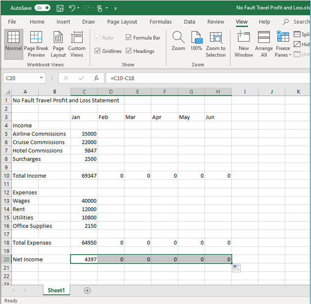
Unless you tell Excel otherwise it will adjust as you copy the formula. For instance, the formula in cell C20 (the net income) is =C10-C18. Copying that formula to cell D20 will cause Excel to change the references from C to D. Once copied to cell D20, the formula would change to =D10-D18. The formula does the same thing when you copy it. It subtracts the total expenses from the total income, in the column you copied it to. Excel adjusts formula when you copy them to fit their new location.

This feature allows you to copy formulas that do the same thing many times. Just remember that the only formulas that can be copied without making adjustments are formulas that will do the exact same thing in relation to the cell with the formula, but in a different location. As in the example discussed in the previous paragraph, the formula is always subtracting a cell two rows above the cell with the formula from the cell twelve rows above that cell, no matter where you copy that formula to.

In the example worksheet, the formulas for total income, total expenses, and net income are all formulas that can be copied because you do want them to do the same computations in the place they are copied to was the formula did when you created it. You will use the fill handle to make the copy process even easier.

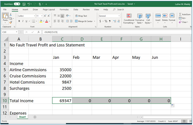
1. Move to cell C10.

2. Locate the fill handle in the lower right corner of this cell.

3. Drag the fill handle to cell H10.

You should now see zeros in the cells where you just copied the formula. As you enter data into the income cells for each month, the formulas will display different values.

4. Use the fill handle to copy the formulas located in cells C18 and C20 to H18 and H20 as shown.

These cells will also display zero values because there are no values in the cells the new formulas refer to. As soon as you add some values for the additional months, the cells with the formulas will display values too.

5. Save the file but leave it open.

Saving the workbook periodically prevents losing data in case of a power outage or computer glitch. Even with the Auto Save feature on, it is a good idea to save manually often, especially after changing something significant or before closing the file, just in case.

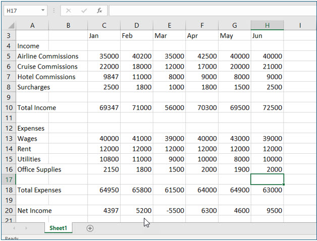
6. Enter the additional values as shown below:

As you enter these values, do not enter anything in the cells with formulas in them. You should notice that the cells with the formulas in them change as you enter values in that column.

7. After entering the data, move to cell A1 with (Control+Home) and then Save and close the workbook.

When you save an Excel workbook, Excel remembers the active cell’s location. Then, when you open the workbook again, Excel takes you to the cell that was active when you saved the workbook. In other words, Excel takes you right back where you were working. You moved to cell A1 before saving so you would be in this cell when you open the saved workbook again.