Using Excel's Goal Seek and Future Value Function

More Excel Topics
Using Excel's Goal Seek and Future Value Function

Using Excel's Goal Seek and Future Value Function

Excel’s Goal Seek feature allows you to specify the outcome you would like in a cell that is a formula then then Excel will adjust a related cell until it finds the outcome you have specified. So, as an example using the Future Value function, you can specify an amount you would like saved for retirement and then have goal seek determine how much you need to contribute and for how long. In this example we’ll have you start with an introduction to the future value (FV) functions and then use goal seek to see what amount you need to save each month to reach your goal.

Watch the video-Goal Seek with Future Value Watch the video-Goal Seek with Mortgage Payment

Using Goal Seek & the Future Value Function – Retirement Scenario

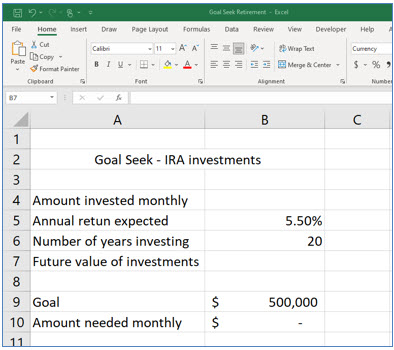
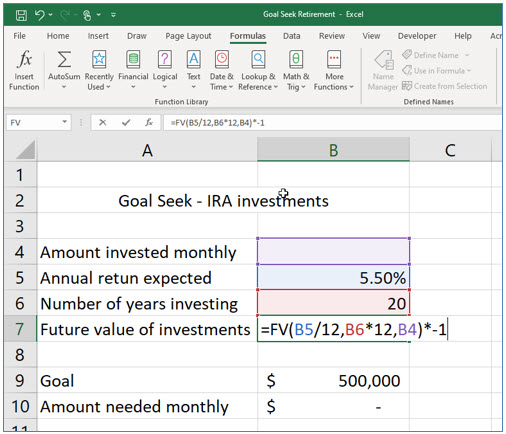
1. Begin by creating the worksheet shown in the image below. You can format the currency and percentage cells as you see fit.

For this example, we are assuming that you expect an average annual return of 5.5% and that you have 20 years before you retire. You can, of course put any values you like in these cells, but maybe after you complete this tutorial. We are also using 500,000 as the target goal.

Using the Future Value (FV) function

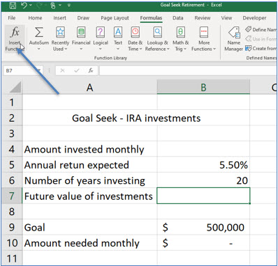
2. Move to cell B7, display the Formulas tab and then click the Insert Function tool.

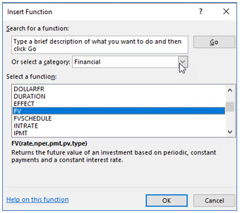
You will now see the Insert Function dialog box. Here you will locate the Future Value function.

3. In the Insert Function dialog box, choose the Financial Category, then scroll down to and select the FV function, then click OK

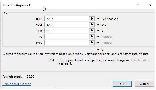
Excel will now display the Function Arguments dialog box. Here you will specify the cells that contain the variables Excel needs to compute the Future Value. Because the amount we are investing is a monthly amount, we need to convert the interest rate and the number of payments into monthly, rather than yearly terms. You will do this by dividing the interest rate by 12 and multiplying the number of payments by 12.

4. Enter the values shown and click OK.

We are leaving the amount we save each month blank. We will have Goal Seek compute the amount we need to contribute each month to reach our goal.

You will now modify the formula to show a positive, rather than negative number. This will make using the Goal Seek feature easier to understand.

5. Click in the formula bar and add *-1 to the end of the FV formula, outside the closing parenthesis.

You can also double-click in the cell with the formula to make this change.

Using the Goal Seek feature

You have set up a working future value template. You can put in your own values and watch the result. The one drawback with this formula is that it assumes the amount contributed each month remains the same. But, knowing that limitation, this is still a very useful function.

You will now use Excel’s Goal Seek to find out how much you need to contribute each month for 20 years to reach the foal of $500,000.

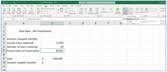
1. Move to Cell B7, select the Data Tab, click the What If tool and select Goal Seek.

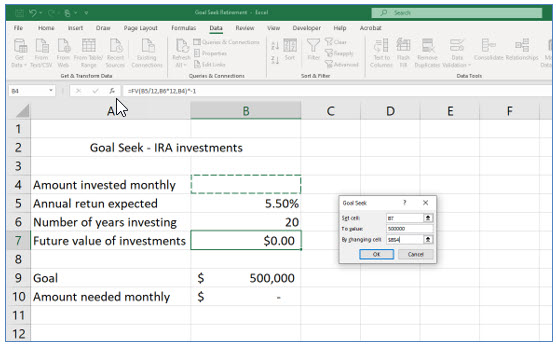
Now you will enter the cells you want to change, the value you want, and the cell that should have that value. The goal seek requires that you “hard code” the value rather than refer to a cell that has the value.

2. In the Goal Seek dialog box, enter B7 in the Set Cell area, 500000 in the To Value area and B4 in the By changing cell area, then click OK.

3. In the Goal Seek dialog box, enter B7 in the Set Cell area, 500000 in the To Value area and B4 in the By changing cell area, then click OK.

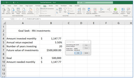
Excel adjusted cell B4 until it reached the goal of $500,000.

4. Click OK to accept Goal Seek’s results.

You have now seen how to use the Future Value function and Excel’s Goal Seek feature. You can now use both in your own applications.