Getting Started With Excel

Note: These instructions are an excerpt of Luther Maddy’s Excel workbooks which are available in printed or eBook format from Amazon.com

Watch the video-Creating Basic Formulas

Microsoft Ecel: Time Saving shortcut keys

Getting Started With Excel

Excel is a spreadsheet program. Spreadsheets are useful primarily for information in which you will perform mathematical computations. Uses for spreadsheets run from simple applications like tracking a family budget, to performing complex financial modeling. One of the advantages of using a spreadsheet is that you can make changes in numeric values and instantly see how that change affects computed values. That allows spreadsheet users to perform “what if” analysis.

Starting Excel

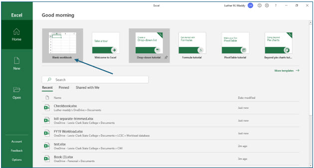
When you start Excel, it allows you to open a workbook you have previously created, create a new blank workbook, or use one of the many pre-defined templates available with Excel 2016. For this course in Excel Basics, you will create workbooks from scratch to allow you to learn more about it. So, the option you want to select when you start Excel is Blank Workbook..

1. Start Excel if needed and select a Blank Workbook at the startup screen.

The Excel Window

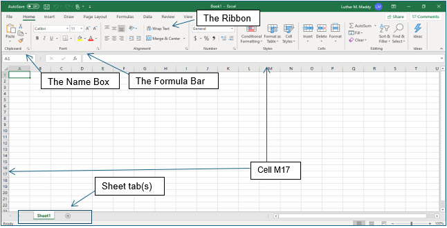
After selecting the Blank Workbook, you should see a new, blank workbook. Here are some of the items you should be aware of when using Excel.

The Ribbon:

The Ribbon displays feature tabs. The ribbon allows you access to features related to the tab name. The most commonly used features are found on the Home ribbon.

The Name Box:

The name box displays the address or reference of the active cell.

The Cell:

You should notice a series of rows and columns. Each of these rows and columns intersect to form cells. Each cell has a unique address or reference. The cell’s address is the column first and then the row. For example, the cell in the top left corner of the worksheet is referred to as A1, column A, row 1. This is verified in the Name Box, or the active cell’s address as we referred to it earlier. The active cell also contains the cell pointer.

The Formula Bar:

The formula bar will display the actual contents of a cell. Cells can contain labels, values, dates and formulas. The formula bar will display what is in the cell, the formula for example. The cell itself will display the result of that formula.

Moving Around the Worksheet

The Excel Worksheet consists of 16,384 columns and 1,048,576 rows. This is a very large area of workspace. While you can use the arrow keys to move cell by cell, this is not very efficient if you are working with a large number of cells. To solve this problem, Excel allows you to move to other cells several ways. Among these are:

Page Down Moves one screen down

Page UP Moves one screen up

Alt+Page UP Moves one screen left

Alt+Page Down Moves one screen right

*How far the active cell indicator actually moves depends on the number of rows or columns you can see on one screen. This is determined by column width, row height and even computer display resolution.

The Go To command

Should you need to move to a cell several screens away, you can use the Go To command. This command will quickly move you to a cell after you type that cell’s address.

You can access the Go To command from the Home Tab  Editing  Find & Select. You can also use (F5) to get to the Go To command. One of the quickest ways to access the Go To command is to click in the Name Box and then type the address of the cell you want to go to and then press (Enter).

Entering Data in Cells

In this portion of the lesson you will enter data types into cells.

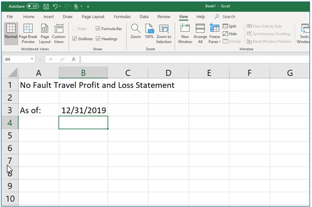
2. In the new workbook, ensure cell A1 is the active cell.

You should see “A1” displayed in the name box and the headings for Column A and row 1 should appear differently than the other row and column headings.

3. In this cell type: No Fault Travel Profit and Loss Statement and press (Enter).

When you pressed (Enter), you should have moved down to cell A2.

Working with Long Labels

The text in cell A1 is called a long label. It is called a label because it is text instead of numeric values. It is called a long label because it exceeds the width of the cell in which you typed it.

Long labels can move into cells next to them as long as those cells are empty. If those cells contain data, then the long label cannot move into that cell. Even though the title you just typed appears to be in several cells, it is actually contained completely in cell A1.

4. Move to cell A3, type As of: and then press the (Right) arrow.

You should now be in cell B3. Pressing a direction key completes the data entry process and moves the active cell indicator in the direction you selected.

5. In cell B3 type 12/31/19 and press (Enter).

You can enter dates in Excel as you would type them. You can also use dates in computations if needed. If this cell displays ##### instead of the date, Column B is not wide enough. You can ignore this for now, you’ll learn to change column width in just a few pages.

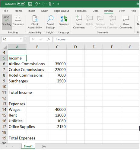
6. Move to cell A5 and enter the remaining data to have your worksheet appear as the one below:

Don’t add any formatting such as dollar ($) signs. You will add formatting in a later lesson. Be sure to enter the data in the cells as shown.

Saving Workbooks

To keep from losing your work you should save at regular intervals. The first time you save you will have to give the file a name. Excel does have an Auto Save feature that will ensure your workbook is saved automatically. Manually saving it the first time allows you to know where the file is stored and what you have named it.

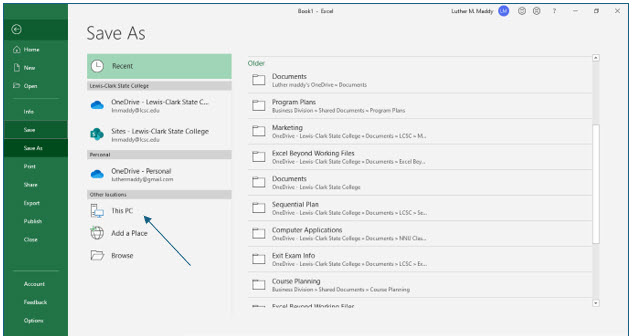
1. Click File on the ribbon to open the File menu, and then choose Save.

Because you have not yet named this file, Excel displays the options for “Save As” rather than “Save”. Here you will tell Excel now where you would like to save this file and give it a name. Where you save your documents may differ, but this course will be assuming you are saving in the Documents folder in Microsoft’s OneDrive. If you want to choose a different location, you may do so easily by clicking the Browse icon and then choosing a location.

2. Choose This PC and then Documents as the location to save this workbook.

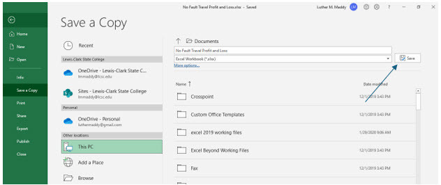
You will now see the Save As dialog box. You will only see this dialog box when you choose the Save command for the first time in a file.

Depending on your version of Windows, your Save As dialog box may appear different than the one above. If you are using a folder other than Documents, make sure you remember where you saved the file so you can find it again.

3. In the File name text box type, No Fault Travel Profit and Loss and then click Save.

You will now return to the worksheet. You should notice the name of the file on the title bar at the top of the Excel window. You can now make additional changes to the spreadsheet and then save it periodically to ensure you do not lose any important work. If the Auto Save feature is on, Excel will save this file automatically for you.

Entering Basic Formulas

Excel is all about formulas and formulas are all about math. Even if you can’t add 2+2, that’s OK because Excel does the math for you. However, when you are creating your own formulas, you will need to use some basic math, such as knowing which math operations you want to perform and what numbers you want to use in the formula.

If you are somewhat math challenged, you will probably finding creating your own formulas easier than trying to understand some of the formulas you create in this workbook. Follow along with the formulas in the exercises and after you’ve made it through, you’ll probably find creating formulas is nothing to fear.

To enter a formula manually, you will begin it with = and then type the formula. The formula should refer to the cell addresses that you want to compute, not the values in those cells. For example, =B3+B4, not =232+343.

You can use the four basic math functions in Excel formulas, Addition (+), Subtraction (-), Multiplication (*), and Division (/). These symbols are easily accessible on the numeric keypad of the keyboard. The other operation you can perform in Excel formulas is exponentiation. That is raising a value by a certain power, such as 32. The exponent symbol is ^ (above the 6 on the keyboard) and is performed before any other calculation in the order of operations.

Order of Operation

When Excel encounters formulas with different operators such as multiplication and addition, there is a certain order in which it performs the computation. To help you remember this order you may try the acronym, “Please Excuse My Dear Aunt Sally”. The order of operation is: Parentheses, Exponent, Multiply, or Divide, before Adding or Subtracting. Multiplication and Division have an equal weight, so if there are both, go from left to right. The same is true for Addition and Subtraction. You can change the order of operation by adding parenthesis, (). When Excel sees parenthesis, it performs that part of the formula first.

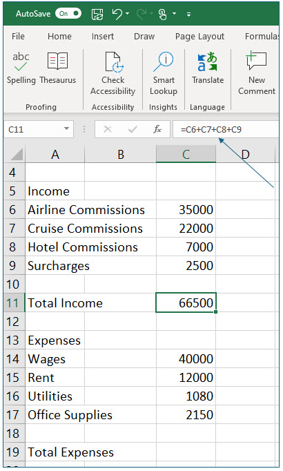
1. Move to cell C11.

You can move here by using the arrow keys or by simply clicking in the cell. In this cell you will enter a formula to add all the income sources together.

2. In this cell type: =C6+C7+C8+C9 and press (Enter)

The = at the beginning of this formula tells Excel that you are creating a formula. You should now see the total of these values in cell C11.

Using Cell Addresses in Formulas

When you create formulas you could just type the values rather than the cell addresses, =123+456 for example. However, entering a formula this way creates the formula using constant values. If you ever changed the values in the cells from 123 or 456 to something else, the formula would not reflect that change because it is always adding 123 to 456. By using the cell addresses, C6, C7 and so on, if the values in those cells change, the cell with the formula will adjust to the new values. If you had “hard coded” numbers into the formula, you would have to change the formula as well as the numbers to have it display the correct values. Whenever possible, use cell addresses in formulas rather than actual values.

Notice the formula you typed is visible in the formula bar. The result is visible in the cell. The formula bar shows you what is actually in a cell, in this case, a formula. The result of the formula is displayed in the cell itself.

The AutoSum Tool

Entering a formula as you just did could be very tedious, especially in cases where you need to add several values in the same row or column. If you have several values in a row or a column that you want to add together, you can then use Excel’s AutoSum tool to create the formula for you. You will now use the AutoSum tool to total the expenses.

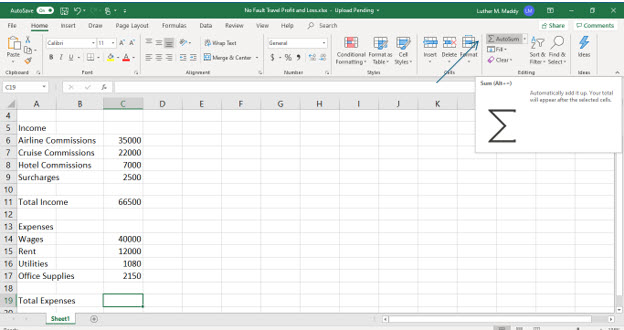
3. Move to cell C19 and click the AutoSum tool on the Home ribbon.

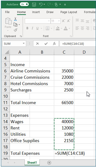
Excel will now place a marquee around the cells it thinks you want to total. In this case, Excel has guessed correctly. In instances where the cells are not correct, you can click and drag to choose the cells you want to add. After selecting the correct cells, you can simply press (Enter) to complete the formula.

4. Press (Enter) to complete the formula.

You should see a total in cell C19.

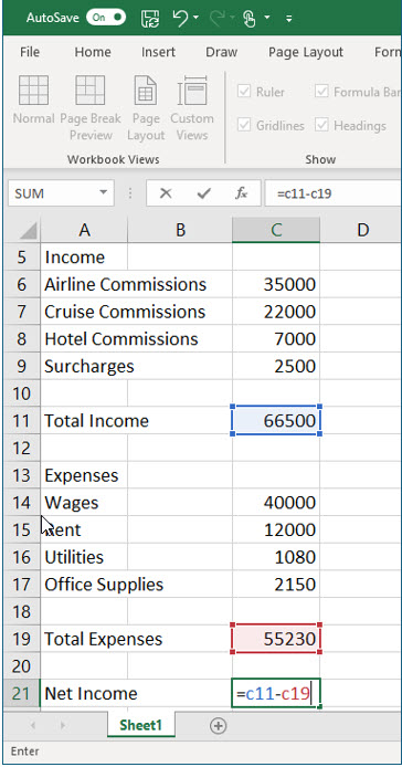
The next formula you create will compute the net income for this example company, No Fault Travel. You will do this by having Excel subtract the total expenses from the total income.

5. Move to cell A21 and type Net Income and then press the (Right) arrow twice to move to cell C21.

6. In cell C21 type =C11-C19 and press (Enter).

The formula you just created subtracts the expenses from the income to compute the company’s profit.

7. Click the File tab and choose Save.

This saves the changes you have just made to the workbook. Notice that you did not have to specify the name again. You only need to give the file a name the first time you save. If you had selected the Save As command, Excel would give you the chance to save the file under a different name. Choosing the Save As command will allow you to confirm that you want to overwrite this file. Using the Save command is the fastest way to continually save a file as you are working on it.

Again, if the Auto Save feature is on, you do not need to do this, but saving periodically is a good habit to acquire for extra protection when you are using programs that do not have the Auto Save feature, or for times when you may have mistakenly turned it off.

You can also use the Quick Access toolbar to save, but just clicking on the icon that resembles a computer disk. You can also see the status of the Auto Save feature here too.

8. Click the File tab and choose Close.

You have now “put away” this workbook and can now create a new one or open an existing workbook. You will do both in the next lesson.

Sponsored Ads

---