Formatting Worksheets
This lesson includes step by step instructions to format cells and worksheets including inserting and deleteing rows and columns, changing column width and rotating text within calls. It also includes adding numeric formatting to cells.
Note: These instructions are excerpted from Luther Maddy’s Excel Workbooks (C) 2024 which are available in printed or eBook format from Amazon.com
Watch the video-Enhancing Cells and Worksheets
Download Excel Formmating Excercise File
Formatting Worksheets
Inserting and Deleting Rows and Columns
If, after nearly completing your worksheet you realize you need additional rows or columns you can easily add them. However, realize that adding a row does so for the entire worksheet. As you add columns or rows Excel will automatically adjust the formulas that need to change. You can also delete columns you may no longer need. In deleting rows or columns you are just shifting your worksheet data up or to the left. The column letter or row number does not disappear, just the information in that row or column. In this lesson you will insert an additional income category in the No Fault Travel spreadsheet.
1. Open the No Fault Travel Profit and Loss workbook.
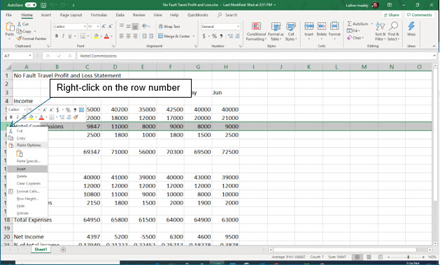
2. Move to the row heading for row 7 and right-click.
You should now see a shortcut menu. This menu allows you to insert additional rows or to delete this row.
3. From the shortcut menu click Insert.
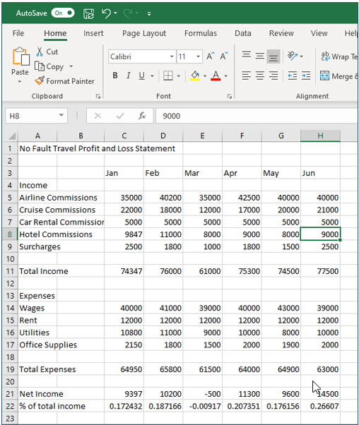
Excel should have added a new blank row and moved all data below row 7. All formulas affected by the addition of this row have been updated automatically by Excel.
4. In the new row 7, type Car Rental Commissions in A7.
Once again you have entered a long label. You will correct this shortly.
5. Enter 5000 for each month for this new income category.
You should notice that the 5000 amount for car rental commissions is also included in the total income. This would not have happened if you had not changed this formula to use the Sum() function. The formula in C11, the total for the month, adjusted automatically to include the car rental commissions.
Changing Cell Alignment
By default, Excel left aligns all labels. You can easily change the alignment of a cell with the formatting tools on the ribbon. For some alignment options you will need to use the Format dialog box. In this portion of the exercise you will change cell alignment.
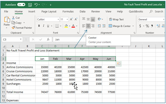
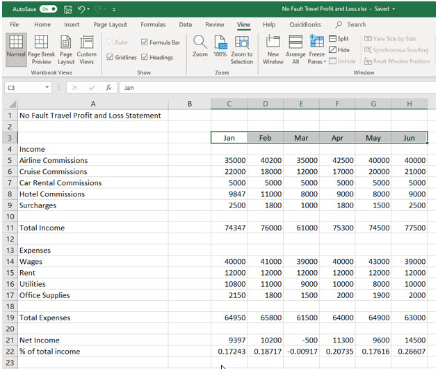
1. Select cells C3 through H3 by clicking and dragging.
2. With these cells selected, locate and click the Center tool on the Home tab of the ribbon.
The labels for each month are now centered in their cells.
Changing Column Width
Rather than having long labels move into neighboring cells, you may want to simply increase the width of the column. Excel provides two basic ways to adjust column width, best fit and manual. With the best fit method, Excel will automatically adjust the column to fit the largest label or value it finds in the column. With the manual method, you decide how wide the column should be by dragging.
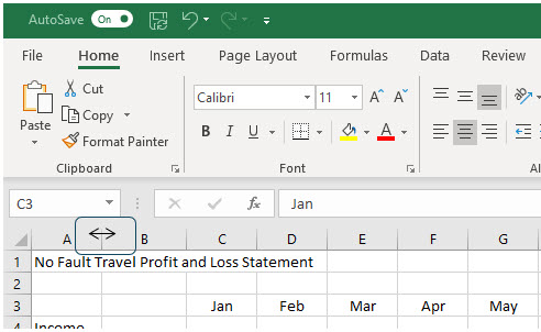
1. Move the mouse between the headings for columns A and B.
When you are in the correct location, the mouse pointer will appear as a black plus with arrows pointing left and right.
2. Double-click between the column headings.
Excel will automatically adjust column A so that the longest label in the column fits. However, adjusting to the longest label in this case makes the column too wide. You will now use the manual method to reduce the size of this column.
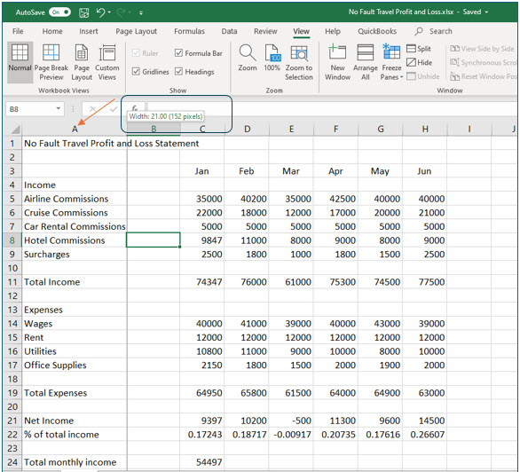
3. Move to the border between the headings for columns A and B. When you see the black plus |, click and drag to the left. Adjust the column to a width of 21.00 characters.
As you drag the column border, you will see the column width appear in a box near the top of the column heading.
Using Merge & Center
The Center command you just used centers cell contents within the cell. This command would have little or undesirable results when used with labels that exceed the boundaries of their cell. If you wish to center a long label within several cells Excel provides the Merge & Center command.
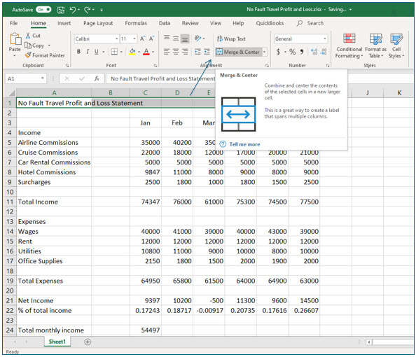
1. Select cells A1 through H1.
To use the Merge & Center command, first select the cells you want the text to be centered within. Remember to use the “white plus” to select cells.
2. After selecting these cells, locate and click the Merge and Center tool on the Home ribbon.
The cells you selected have now become one large cell. The heading is now centered in the new larger cell.
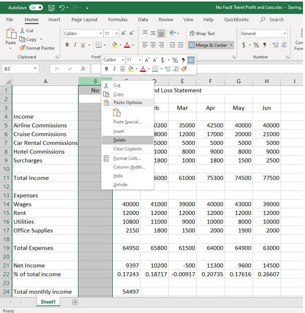
Column B is now an “extra” column. You’ll now delete this column and, as you do this, Excel will automatically adjust all the formulas so they will still work.
3. Right-click column B’s heading and choose Delete from the shortcut menu.
After you clicked Delete, Excel essentially moved all the other data over one column. You should notice all the formulas still compute correctly.
Rotating Text
Excel provides a very easy way to rotate text. This makes it very easy to create impressive spreadsheets.
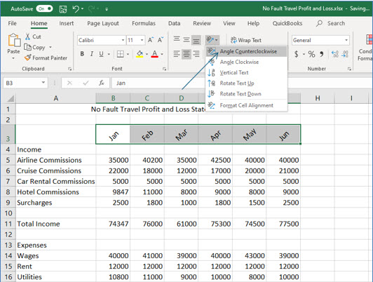
1. Select cells B3 through G3.
You will rotate the month names in this worksheet.
2. Click the Orientation tool in the Alignment group.
3. Select Angle Counterclockwise.
The month names should now be rotated 45 degrees.
Numeric Formatting
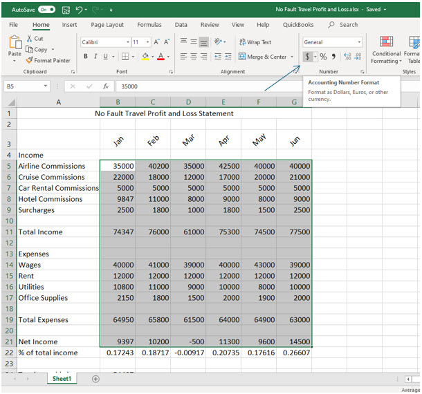
Excel has several numeric formatting options that you can easily add to values. You can access accounting (currency), percentage, and comma formatting from the ribbon. Several other numeric and date formatting options are available from the Format Cells dialog box.
1. Select cells B5 through G21 and then click the Accounting style tool ($) in the Number group in the Home tab on the ribbon.
The values in the cells you selected should now appear with currency formatting.
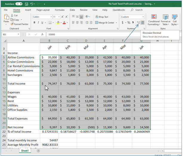
The default accounting style adds both dollars and cents. In this case an even dollar amount is all you need to see. You will now change the formatting to display no values to the right of the decimal point.
2. Leaving the cells selected, locate and click the Decrease Decimal tool in the Number group twice.
You should now see the numbers displayed in even dollar amounts.
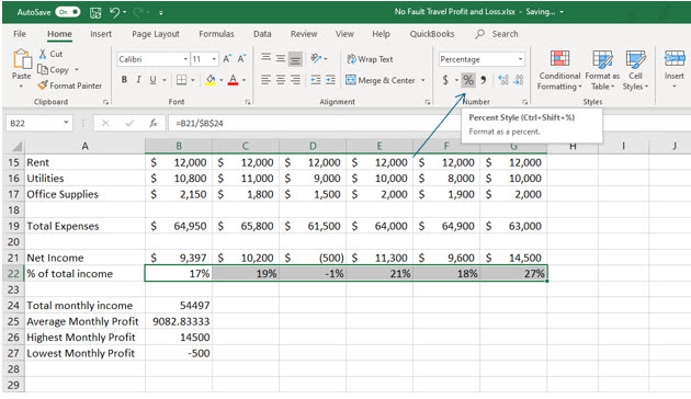
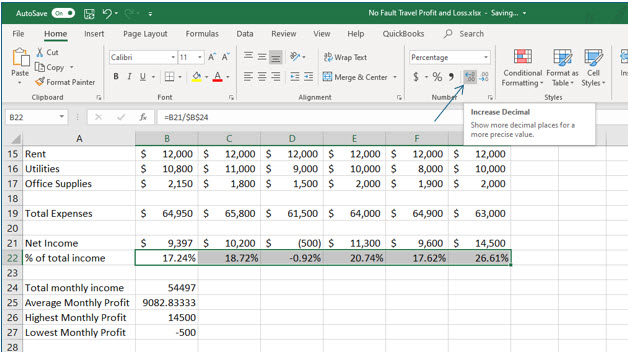
Now you’ll add percentage formatting to the percentages you computed using the absolute reference feature.
3. Select cells B22 through G22.
4. Click the Percent style tool in the Number group on the Home tab of the ribbon.
You have now added percentage formatting to these cells. You’ll now add two decimal places to increase the accuracy of the percentages.
5. Leaving these cells selected, locate and click the Increase Decimal tool in the numbering group of the Home tab on the ribbon twice.
The percentages now display more accurately with two decimal places.
6. Add Accounting ($) formatting to cells B24 and B27.
This time you’ll leave the display at two decimal places for accuracy to the penny.
7. Save and close the workbook.
