Using Excel's Filtering and Subtotals
This lesson explains how to use Excel’s filtering and subtotaling feature to quickly and easily summarize large data sets.
Note: These instructions are excerpted from Luther Maddy’s Excel Workbooks (C) 2024 which are available in printed or eBook format from Amazon.com
Watch the video-Using Excel's Filtering and Subtoal features
Download TripData to complete the lesson
Creating Automatic Subtotals
When you are dealing with many records, Excel’s Subtotal feature allows you to group and summarize values in that data. You can perform basic statistical functions such as sum, average, or count for groups of records, such as by trip destination with this example. You can also use Excel’s subtotal feature to create slightly more complex statistical analysis by computing standard deviation and variance.
To “group” the records, you will first need to sort the records by the field you intend to group on.
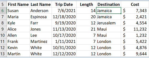
1. Click in the Destination field. In the Sort & Filter group on the Data tab, use the Sort A to Z button to sort the records based on the Destination field in ascending order.
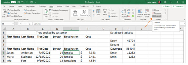
2. Be sure the active cell is within the database. Click the Subtotal tool in the Outline group on the Data tab.
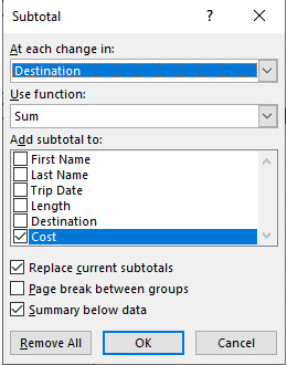
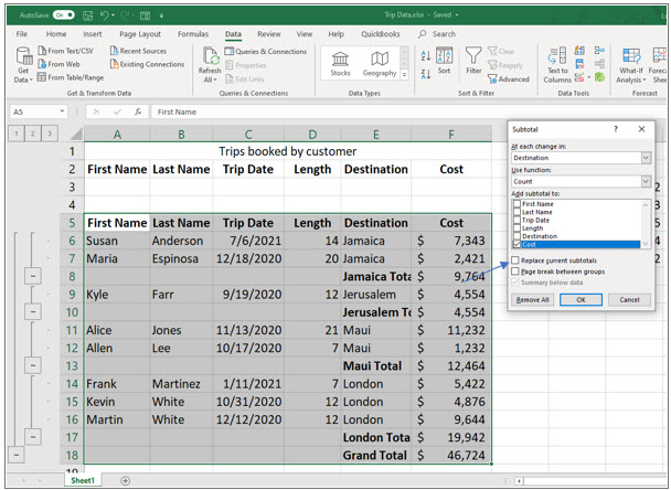
In the Subtotal dialog box, you will select which field determines how the records are subdivided. You will also select which computation will be performed (i.e., sum, average, etc.) and which field values will be used in the computation.
3. Select Destination in the At each change in text box (which establishes the groups).
This tells Excel to compute a subtotal each time the Destination field value changes. You sorted the records by destination in ascending order so the destinations would be grouped together.
4. Select Sum as the function. Select Cost as the field to Add subtotal to; these values will be used in the computation.
Leave the other options as shown.
5. Click OK
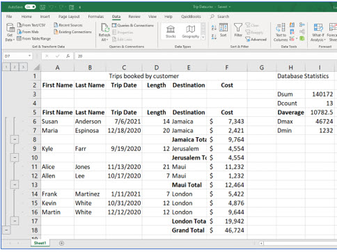
Your worksheet should look like the one below. You should see a total computed for each destination. Did you notice that the Subtotal tool was in the Outline group when you selected it? Do you remember when we experimented with outlining in the Excel: Beyond the Basics course that preceded this one? Notice the outline level numbers and controls left of the column headings and row numbers. We will explore these next.
Expanding and Collapsing Subtotals
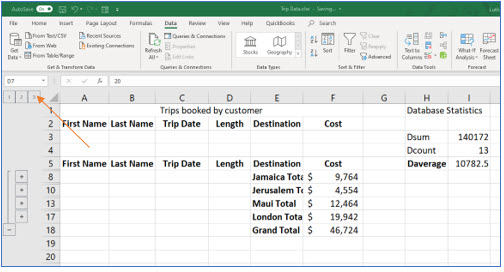
The Excel workbook currently shows all records (details), group totals (subtotals), and the grand total (summary). You can click on the outline level numbers 1, 2, or 3 to see just the grand total (level 1), the grand and group totals (level 2), or all information (level 3). You can also click on the outline buttons to the left of the row numbers. The level 2 buttons (+ or -) will expand or collapse the group records, but not the subtotals.
1. Click on the “2” to the left of Column A’s heading.
Excel should now show the subtotal for each destination and the grand total.
Experiment with the various outline levels. Also look at the worksheet in Print Preview; the worksheet will print as it is displayed on screen.
Adding more subtotals
The subtotals you created added a sum or total for each destination and a grand total. This is because you selected Sum as the subtotaling function. If you decided that you wanted the record count instead of the total, you could click the subtotal tool again and choose Count instead of Sum. By default, Excel will replace the Sum computations with a count.
However, there may be times when you want two computations to display on the worksheet when you are using the Subtotal feature. In this portion of the lesson you will add a Count for each destination, but leave the Sum as it is.
2. Ensure the active cell is located in the database area and click the Subtotal tool again.
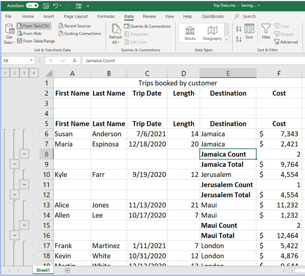
3. In the Subtotal dialog box, change the function to Count. Then turn off the Replace Current subtotals check box and click OK.
You should now see that Excel added the count and the total to the worksheet. Adjust the destination’s column width if needed to see the complete titles.
Removing Subtotals
Changing the computation to be performed on the grouped items or removing the subtotals is simple with the Subtotal dialog box. To change the computation, just click on the Subtotal tool when any cell in the database is active. You might try changing the computation to group averages and grand average for our current database.
1. With the active cell in the database area, click the Subtotals tool in the Outline group on the Data tab.
The Subtotal dialog box should appear.
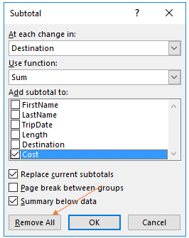
2. In the Subtotal dialog box, click Remove All.
Excel will now remove all subtotals (the group and grand totals) calculated for the database records.
