Enhancing Worksheets
This lesson includes step-by-step instructions to teach you to add shading, borders, and colors to cells in Excel. It will also show you how to use the Format Painter tool.
Note: These instructions are excerpted from Luther Maddy’s Excel Workbooks (C) 2024 which are available in printed or eBook format from Amazon.com
Watch the video-Enhancing Cells and Worksheets
Download Excel Enhancing Exercise File
Enhancing Worksheets
It is very easy to enhance cells in an Excel worksheet. To enhance cells, first select the cells you wish to enhance. Then, select the enhancement you need either from the ribbon or from the Format dialog box.
1. Open the No Fault Travel P&L workbook.
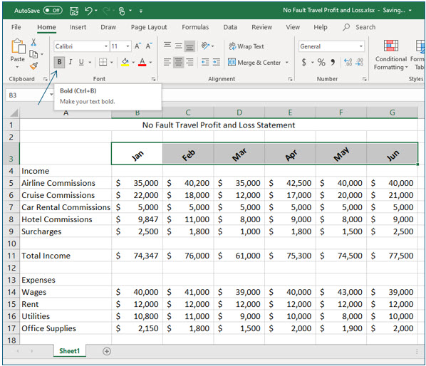
You’ll now add boldfacing to the month names in this worksheet.
2. Select cells B3 through G3 and then click the Bold tool on the Home tab of the ribbon.
The labels in these cells should be boldfaced.
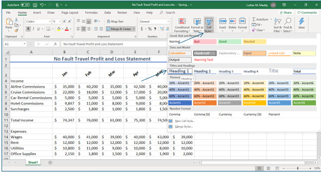
Now, you’ll use a built in Excel style to format the title in cell A1.
3. Move to cell A1 and click the Cell Styles drop down list. You can find this tool in the Styles group on the Home tab.
4. Choose Heading 1 from the styles list.
Cell A1 should now be formatted in the Heading 1 style. You may not see this style until you move away from cell A1.
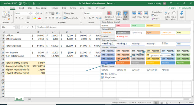
You’ll now apply a shading cell style to the statistical calculations at the bottom of the worksheet.
5. Select cells A24 through B27 and then click the Cell Styles drop down list.
6. From the list of cell styles, choose 20%-Accent4.
These cells will now be shaded in light orange.
7. Apply Accounting style formatting to cells B24 through B27.
Adding Cell Borders
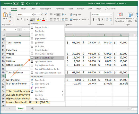
To further set off or enhance cells you can easily add borders to cells. You can add top, bottom, left, right, or all four borders. In this portion of the exercise you’ll use the Border tool to add a border to the row of cells just above the net profit values.
1. Select cells A20 through G20.
This is the empty row of cells just above the net profit.
2. Click the Borders drop down list and choose Bottom Double Border.
You will not see the border until you click outside the selected cells. When you do, you should see that Excel has added a double border to those cells.
Using the Format Cells Dialog Box
Excel allows you to change the font face and size. You can also change the color of the text within cells. You can do this from the ribbon. However, using the Format Cells dialog box allows you to preview the font change before actually applying it. You’ll now use the Format Cells dialog box to make several changes to some of the cells in this worksheet.
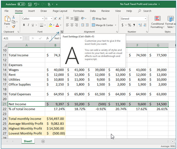
1. Select cells A21 through G21 then click the Format cells dialog box launcher in the Font group of the Home tab.
Excel will now display the Format Cells dialog box. Here you can choose from many more formatting options than are available directly on the ribbon.
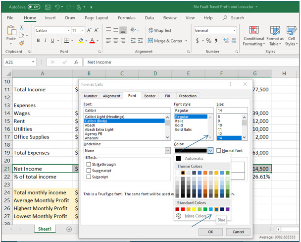
2. Change the font size to 14 points. Then, click the Color drop down list and choose Blue.
After choosing the color, notice that the preview lets you see how the text will appear.
3. Click OK after making these changes.
The net income text should now appear with the enhancements you specified. You will see these changes when you move away from the selected cells.
4. Select cells A19 through G19, the total expenses row.
You will now shade and add line options around to these cells.
5. Launch the Format Cells dialog box.
While the exercise step had you use the Font group, you can launch this dialog box from the Font, Alignment, or Number groups.
Shading Cells
Excel also allows you to add shading to cells or a group of selected cells. When you do add shading to your own worksheets, just be sure to choose a color that will not be so dark that you cannot see the information in a shaded cell.
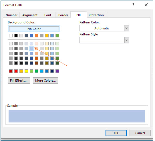
6. Click the Fill tab in the Format Cells dialog box.
7. Choose light blue for the fill color and then click the Border tab.
Leave this dialog box open for now.
Cell Borders
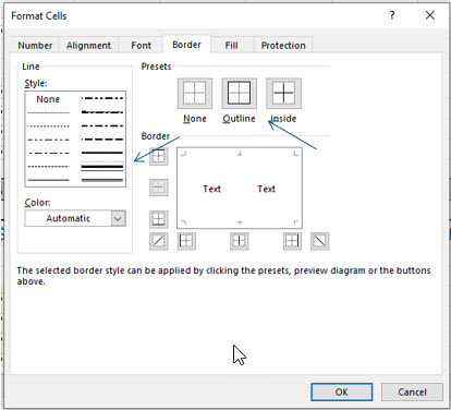
You can also add lines or borders to selected cells from this dialog box. When you enter the Borders tab in the Format Cells dialog box you can choose a line style and also choose where and how you want that line style applied.
1. In the Border tab, choose the sixth Line Style down in the second column.
2. After choosing the Line Style, click the Outline button and click OK.
You have now informed Excel to place a line around the cells you have selected. If you click anywhere outside the selected cells you will see this change.
The Format Painter
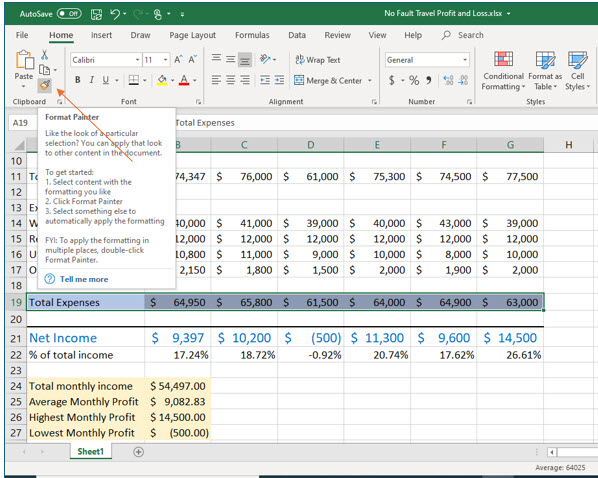
The Format Painter allows you to copy formatting options from one cell to another cell or group of cells. For instance, you just added borders and shading to the cells in row 19. If you want other cells to look the same way, you can use the Format Painter to copy that formatting.
1. Select cells A19 to G19 again.
The first step in using the Format Painter is to move into a cell that has the formatting options you want to copy. This could be a single cell, but since this group of cells has a border around the entire group, you need to select all the cells to duplicate the outside border around all the cells you are about to select.
2. Click the Format Painter tool in the Home tab.
After clicking the Format Painter tool, Excel will apply the formatting to the next cells you select.
3. Select cells A11 through G11.
You should notice Excel added a paint brush symbol to the mouse pointer.
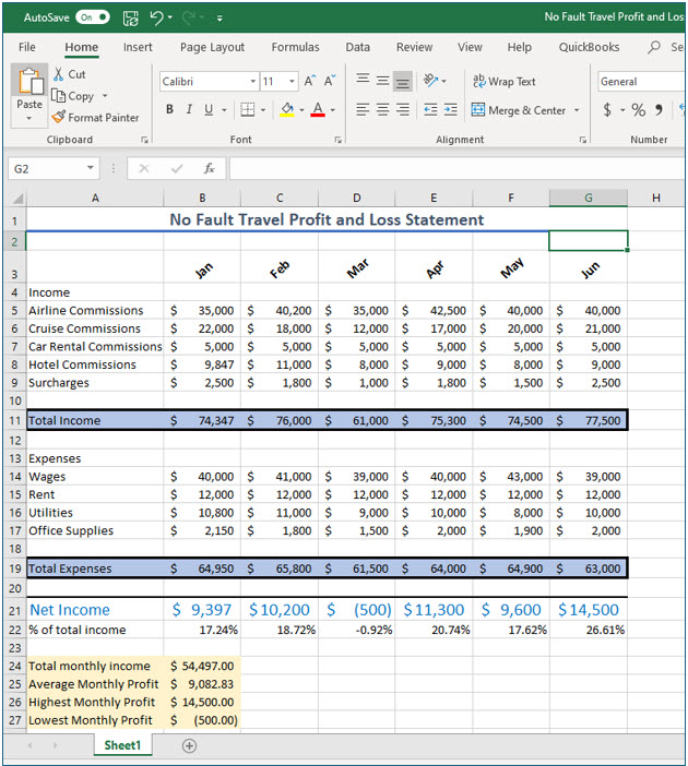
Your worksheet should now appear similar to the above after adding the cell styles and other enhancements.
4. Save and close this workbook when done.
