Excel Database Functions
Note: These instructions are an excerpt of Luther Maddy’s Excel Database and Statistical Features. This full text is available in printed or eBook format from Amazon.com
Excel’s database function library includes many functions that allow you to perform calculations on the data in your Excel database based on conditions (criteria), you specify. For example, the DSUM function will sum values from database records that meet the criteria you specify. In the No Fault Travel database, you could use the DSUM function to total to costs of all the trips to a certain location. You could also get even more specific with criteria and only sum the trip costs to one location and a specific travel date. When you use the database functions, you can specify criteria for one field, several fields, or all fields in the database if you choose.
Watch the video-Creating a loan amortization schedule
Download TripData to complete the lesson
Creating a Criteria Range
Database functions require an area in the worksheet, called the criteria range, where you will set the criteria or conditions which must be met for the record to be included in the result (i.e., which records to include in the sum, average, etc.).
The criteria range must consist of at least two cells: one cell containing the field name and the cell below specifying the condition. Although we will not use it in this exercise, including two blank rows in the criteria range below the field names give you the ability to create “or” options in the Criteria. For instance, you could select Maui or Hanoi by using two rows below the field names in the criteria area.
You will now create a criteria range that includes all the fields in this database. This will allow you to specify conditions for any field. It is perfectly fine to leave field criteria empty. It is also allowable to create a criteria range that only has one or two fields. This will more sense as we progress through this lesson.
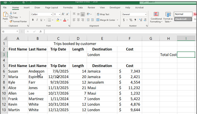
1. Open the Trip Data workbook on this website or create one similar to that shown.
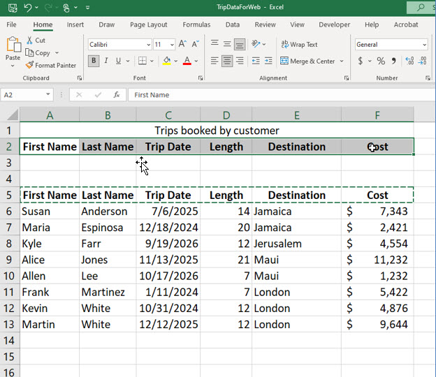
2. Select the field names in cells A5 through F5 and choose Copy.
You are going to copy all the field names to create a criteria range. As we mentioned before, this will allow you to specify conditions (criteria) for any or all of the fields in this database. If you were only concerned about the date and destination, you would only need to copy those two field names.
3. Paste the copy of the field names at cell A2.
You can place the criteria range anywhere. We mainly placed it above the database here to show everything on one screen in this book.
Naming Ranges
Excel allows you to name a specific cell or group of cells. A name is easier to remember than cell addresses. The database records are located in cells A6:F14 and our criteria is located in cells A2:F3. It will be much easier to refer to the database or criteria in formulas if we name those locations. Furthermore, named ranges are absolutely addressed in formulas, so the formulas can be copied without losing the correct cell addresses.
In this part of the lesson, you will name the cell ranges for the criteria and database.
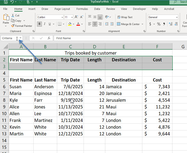
1. Select cells A2 through F3.
This is the criteria range, which includes the field names and a row to specify conditions for each field. If you included one more row, as we mentioned previously, this would allow you to perform “or” specifications.
2. Click in the Name box, type Criteria and press (Enter) to name this range.
You must press (Enter) to assign the name to the selected cells. Clicking outside the name box will not set the range name. You have named these cells “Criteria” and can refer to them by that name in any formulas you create. Excel does not allow spaces in range names, so be sure not to accidentally add a space after typing the name.
Now you will name the range of cells that contain the data, Database.
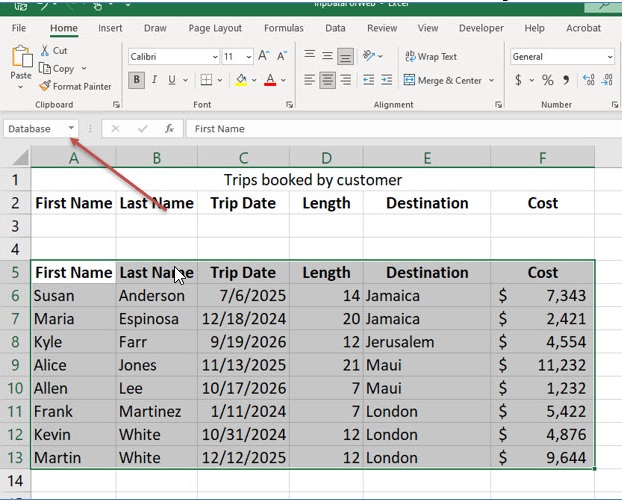
3. Select cells A5 through F13. Click in the Name box and name these cells Database, pressing (Enter) when done.
When you are working with your own data, you can name the criteria and database ranges anything you like. We are using these names just to emphasize the ranges Excel uses in database functions.
Using the DSUM Function
The DSUM function will sum the values in the database for the records that meet the criteria you provide in the criteria range. If you change the criteria, Excel will instantly recalculate the sum based on the new criteria.
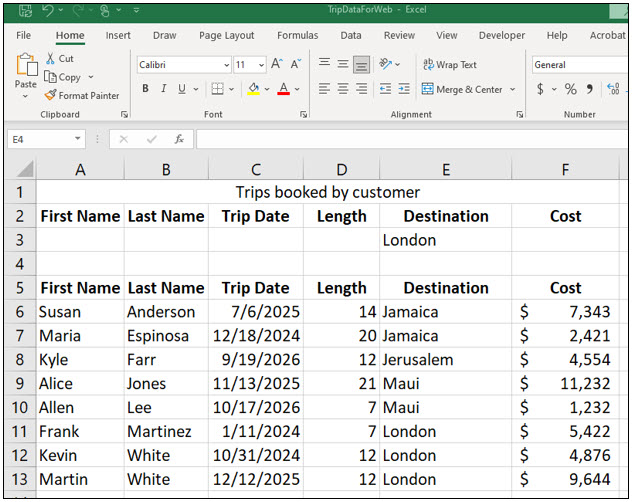
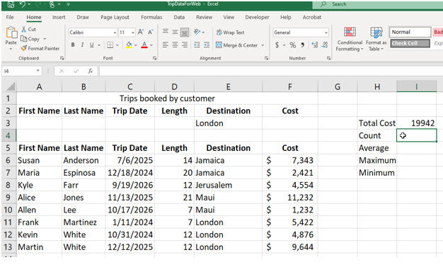
1. Move to cell E3 and type London.
You have set the criteria to be all records with a destination that matches London.
2. Move to cell H3, type Total Cost and then move right to cell I3 (column I, row 3).
When using these functions on your own, you will likely place better descriptions for these values. You are using “DSUM” as the label to remind you what function you used to compute the values. You will place the formula in cell I3.
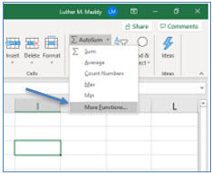
3. In cell I3, click the drop-down list button on the AutoSum tool in the Editing group on the Home tab. Choose More Functions… to display the Insert Function dialog box.
You could have also clicked the Insert Function tool on the formula bar. Microsoft often provides more than one way to select a command in Excel and its other programs.
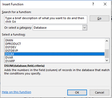
4. In the Insert Function dialog box, choose Database as the Function Category and DSUM as the function. Click OK.
5. In the DSUM dialog box, type Database in the Database text box. Type Cost in the Field text box and Criteria in the Criteria text box. Click OK..
You have used the names you assigned to the cell ranges instead of specifying cell addresses. Excel had added quotation marks to the field name in the Field text box, as “Cost” for you. If you do not use the Function Arguments dialog box, be sure to use quotation marks around the field name (a text label) if you directly type the formula into the cell. You can also enter the cell address (F6, in our case) or the column number in the database (6, in our case) in the Field text box or for the field argument in a formula directly. The field must contain a value type which the function can use in its operations. The database statistical functions (sum, average, count, etc.) require that the field contain a number or a date to return a valid response.
You should now see that Excel had added the cost of all trips taken to London.
6. In cell H4 type Count. Below this, type the rest of the labels as shown below:
These are the other database functions you will use in this lesson.
7. Use the Insert Function tool to enter, in column I, the formulas which correspond to the database functions listed in column H.
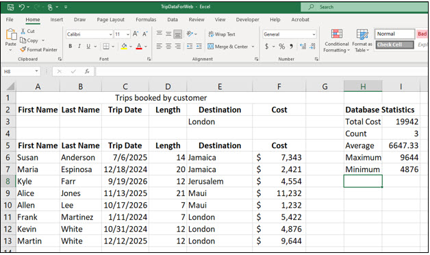
These functions are also categorized as Database functions. Some tips to remember when using the Function Argument dialog box for the database functions: Use the names you assigned to the database and criteria ranges in the Database and Criteria text boxes. Use “Cost” in the Field text box. When you have finished, the statistical values for trip costs should appear in the worksheet with London as the trip destination (which is the criteria you set). The correct values are shown:
8. Add the label Database Statistics in cell H1. Change the alignment of this cell to Left if needed.
Specifying Criteria
The formulas you created incorporated the criteria (or condition) to perform calculations for only those records with London in the destination field. If you change the criteria, Excel will recalculate the statistics based on the new criteria you set.
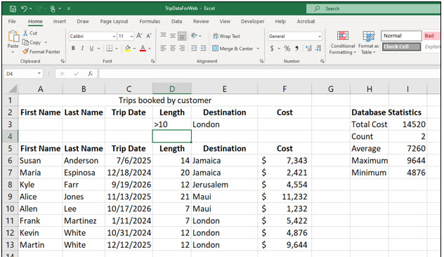
1. Move to cell D3 and enter >10 in this cell. Move out of this cell when done.
Notice that the statistics changed when you changed the criteria. Verify the new values make sense.
You have now specified that only trip records with a London destination and with a trip length greater than 10 days should be included in the statistical calculations. You have simply added an additional condition. Excel treats conditions in multiple fields in the criteria range as “and” conditions. So, you potentially restrict the number of records used in the calculation with each condition you add as all conditions must be met.
2. In Cell E3 press (Delete) to erase the contents of this cell, London.
Make sure you use the delete key instead of putting a space in this field. The statistical values using the Database functions should again change.
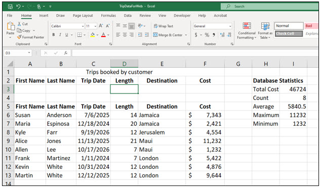
3. Delete the contents of cell D3.
The criteria range is now empty. The values computed with the database functions are displaying statistics for the entire database because you have no conditions specified.Here, the database statistical functions are working just like Excel’s regular statistical functions (i.e., DSUM like SUM, etc.).
4. Move to cell A3, the first name criteria, and enter A*.
You have now used the wildcard (*) in the database criteria. Excel interprets the wild card as “anything,” so A* is a text label beginning with the letter A and anything after the first letter. You have specified all records with a first name beginning with the letter A. Excel will have computed values for only the records that met this criteria.
5. Delete the contents of cell A3.
Once again, the statistics are calculated for all database records because no criteria has been imposed.
6. Save and close the workbook.
You have now seen how easy it is to use Excel’s Database functions to analyze datasets of any size.
