Creating PivotTables
PivotTables are a very versatile and flexible tool to quickly analyze and summarize data in an Excel worksheet. Pivot tables allow you to perform statistical analysis on large Excel databases without having to create any formulas on your own. PivotTables can quickly produce different computations according to your specifications. For example, with our No Fault Travel database, you can have the PivotTable compute the average trip cost to each destination; then, with just a couple of mouse clicks, the PivotTable could display the average cost of a 7-day trip.
Note: These instructions are an excerpt of Luther Maddy’s Excel Database and Statistical Features. This full text is available in printed or eBook format from Amazon.com
Watch the video-Creating and Using Pivot Tables
Downlaod Example File for pivot table Lesson
Creating PivotTables
In this lesson you will use a PivotTable to analyze the database we created for the No Fault Travel Agency.
1. Open the Trip Data workbook.
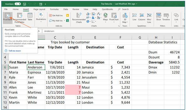
2. Move into the database. In the Tables group on the Insert tab, click the PivotTable tool.
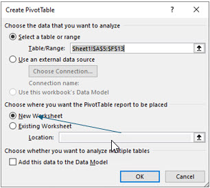
In the Create PivotTable dialog box, you will specify the location of the source data. Since one of the database cells was active when you clicked the PivotTable tool, the database location appeared as the selected data range in the dialog box when it opened. In this dialog box, you will also specify the location for the PivotTable. We will place it in a new worksheet for the same reasons that we have placed charts on new worksheets.
3. In the Create PivotTable dialog box, be sure New Worksheet is selected. Click OK.
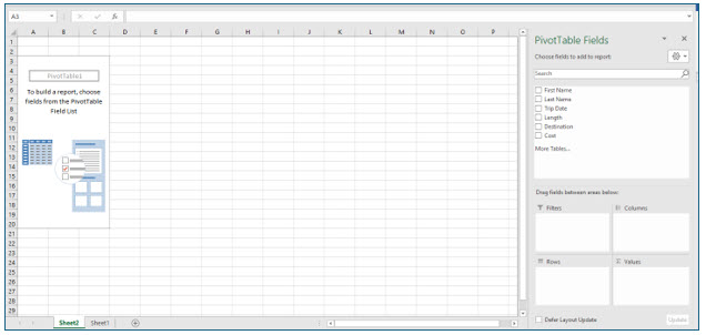
Excel has now created a new worksheet and named it Sheet2. This is a pivot table worksheet and, as of right now, displays no data.
The next steps will be to build the PivotTable by specifying the field containing the values to be used in the computations and the field containing the separate categories (i.e., the groups) that you want to see the computations for.
In the PivotTable Fields task pane, you may simply click a checkbox beside the field name; however, dragging the field to the desired task pane area will ensure that the PivotTable is designed exactly as you wish.
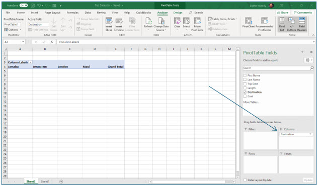
4. In the PivotTable task pane, drag Destination from the field list into the Columns area.
If you had clicked on the Destination rather than dragging it, Excel would have placed the destinations as row headings rather than column headings.
Now, each destination should appear as a column in the PivotTable. The destinations are really serving as the “groups” you created when you used the Subtotal command.
Excel will perform the calculations for each destination.
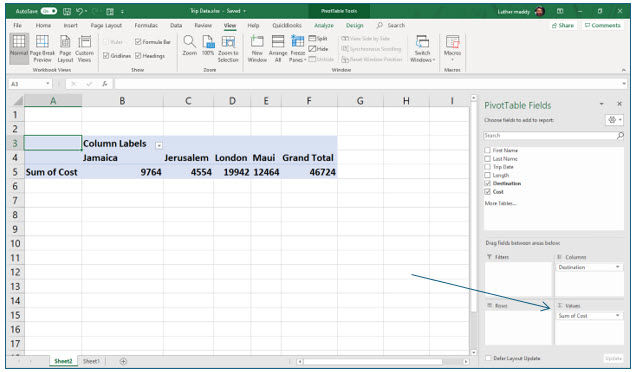
5. Drag Cost from the field list into the Values area in the PivotTable Fields task pane.
Because Excel recognizes the Cost field as a field it can perform calculations with, you would have simply clicked on its checkbox.
The trip cost for each destination should appear in the PivotTable, as well as the grand total for all trips. Be default, Excel uses the Sum function for fields in the Values section. When you dragged Destination to the Columns area in the task pane, Destination was added under Columns. However, when you dragged Cost to the Values area, Sum of Cost was added under Values. This allows you to see what computation Excel is performing on that field.
Changing the Function
If you would like to see the average trip cost to each destination, you can use the Average function instead of Sum in the PivotTable. You can change the computation performed from the Values area of the task pane, or by double-clicking on “Sum of Cost” in the PivotTable.
1. Double click on “Sum of Cost” in the 2nd row of the PivotTable (cell A5).
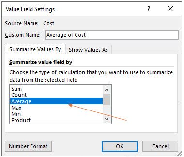
The Value Field Settings dialog box will allow you to choose from about a dozen computations (functions) which can be performed; you can also select number formatting for the result. From the Show Values as tab, you could choose to display the total trip cost for each destination as a percentage of the total cost for all trips.
2. Under Summarize value field by in the Value Field Settings dialog box, choose Average. Then click the Number Format button.
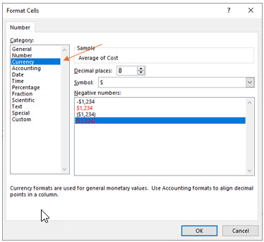
3. In the Format Cells dialog box, choose Currency format, with zero decimal places and then click OK. Click OK again to leave the Value Field Settings dialog box.
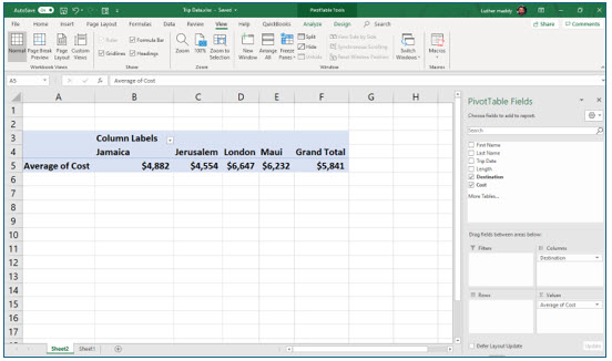
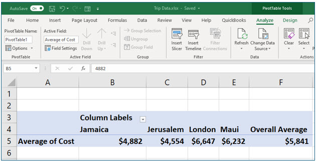
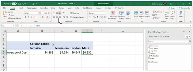
Notice that the PivotChart is now displaying the average trip cost for each destination, not the total cost. The “Grand Total” is really the “Overall Average” for all trips. Also notice that the numbers are formatted with dollar signs ($).
Modifying a PivotTable
After completing a PivotTable, you can still add, change, or remove fields. In the next steps, you will see how easy it is to modify a PivotTable.
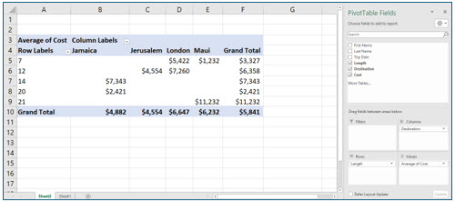
1. Make sure the PivotTable is active. From the field list in the PivotTable Fields task pane, drag Length into the Row area.
Reminder: You can select (i.e., make active) any PivotTable, database, or named range by clicking in one of its cells.
The values from the Length field should appear under the heading “Row Labels” in the PivotTable, which displays the average cost for each trip length and every destination. If you wish to remove a specific destination or only include trips lasting so many days, you can apply a filter to the pivot table.
In this portion of the lesson you will explore using filters within PivotTables.
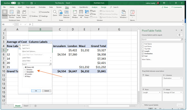
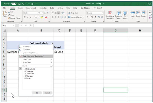
2. In the PivotTable, click the drop-down button in Column Labels.
The destinations are the column labels. The drop-box menu lets you select which destinations to display.
3. Turn off the checkbox for Jerusalem and Jamaica. Click OK.
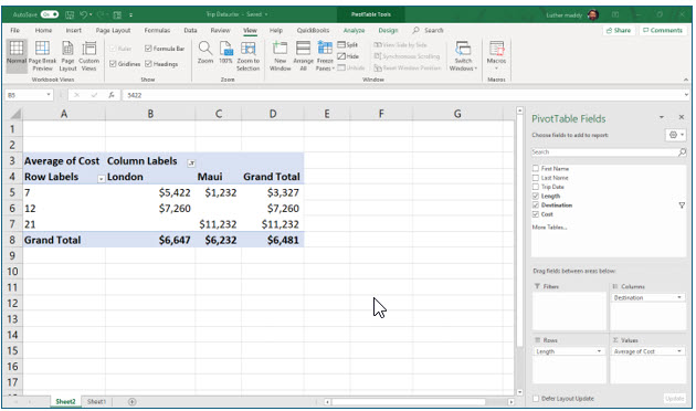
All destinations except the two you de-selected are now shown in the PivotTable. Also notice that the averages have been recalculated. The “Grand Total” (really the overall average) is higher with the trips to Jamaica and Jerusalem removed.
4. Click the drop-down button in Column Labels. Select Clear Filter from “Destination.”
In the next step, you will remove the Length field from the PivotTable.
5. In the PivotTable Fields task pane, de-select (uncheck) Length in the field list.
The pivot table no longer displays the length of the trips.
Changing PivotTable Options
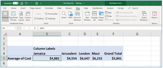
In this portion of the lesson you will learn to turn off the Grand Totaling feature. However, if you want to keep the overall average, you could edit the text in cell F4 from Grand total to Overall Average as shown. However, for this example, we will assume you do not want to display this column in the pivot table.
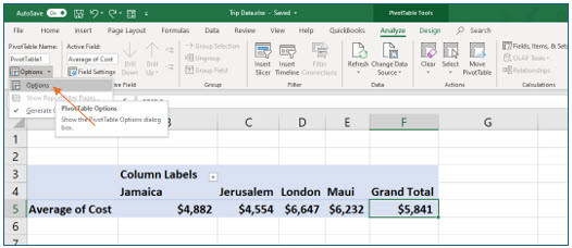
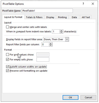
The PivotTable dialog box (shown on the next page) provides many advanced options, which include formatting, filtering, and selecting what is displayed on the PivotTable. For example, you may decide not to display the last column, “Grand Total,” since the caption is misleading when the table displays averages and not totals (i.e., sums). The PivotTable Tools Analyze tab provides access to some of the more advanced features available for PivotTables.
1. Display the Analyze tab on the ribbon and click the Options tool in the Pivot Table group.
You should now see the PivotTable Options dialog box.
2. In the PivotTable options dialog box, select the Totals & Filters tab. Under Grand Totals, de-select the Show grand totals for rows and also turn off Show grand totals for columns. Click OK.
This pivot table currently does not display grand totals for columns, but if you added another field to serve as row headers, the totals would appear for each column, unless you turned off that option too.
The PivotTable should no longer display the “grand total” for all destinations.
Using the Slicer
In this portion of the lesson, we will use the Slicer which is an easy way to filter PivotTable information with a single mouse click. In the next steps, you will add a Slicer for the Destination field to the PivotTable and then use it to choose which destinations appear on the PivotTable.
1. Ensure the PivotTable is active. In the Filter group on the PivotTable Tools Analyze tab, click the Insert Slicer tool.
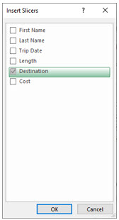
The Insert Slicers dialog box should appear, and as the name implies, you can insert more than one slicer tool for the PivotTable.
2. On the Insert Slicers dialog box, turn on the Destination checkbox and click OK.
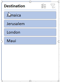
The title of the Slicer is the field (in our case, Destination) that you selected and the buttons on the Slicer are the values contained in that field. For our No Fault Travel database, the Destination slicer is the list of destinations for the booked trips. The Slicer is a filtering tool; the PivotTable will display the computation for the one or more destinations that you select.
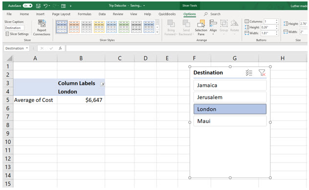
3. If needed, move the slicer so the entire pivot table is visible, then, click London.
With just one click, you have “sliced” the records so that the PivotTable only shows the calculation for the destination you selected. Notice that the destination(s) for the shaded buttons appear on the PivotTable. You can use “Control+Click” to add multiple destinations.
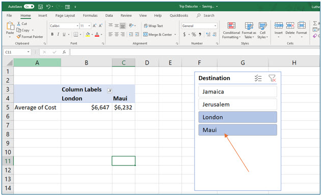
4. Press and hold (Control), and then click on Maui.
Both the London and Maui locations should appear on the PivotTable now.
You could use the Clear Filter button in the top right corner of the slicer to remove the filter and to display all destinations. However, we will remove the filter directly from the PivotTable in the next steps.
5. If sizing handles are not visible on the slicer window frame, click somewhere in a blank area of the slicer.
Sizing handles, small white circles on the frame corners and midpoints, indicate that the slicer window is selected. You can grab any of the sizing handles to resize it. When the slicer window is selected, you can also move it by clicking in any blank area and dragging it. You might want to experiment with resizing and moving now.
6. Press (Delete).
You have removed the Slicer from the pivot table. Excel working environment, but you have not deleted the filter that you applied using the Slicer tool.
7. Click the Filters button on Column Labels in the PivotTable. Choose Clear Filter from “Destination.”
8. Return to sheet1, the data you used for this pivot table. Save and close the workbook.
The PivotTable is saved as a worksheet in this workbook.
