Helpful Excel Features

More Excel Topics
Helpful Excel Features

Helpful Excel Features

This lesson includes step by step instructions to use some of Excel's very helpful features inlcuding outlining, freezing panes, data validation, using cell comments, and protecting worksheets.

Watch the video-How and Why to Freeze Panes Watch the video-Use Data Validation to "user proof" your worksheets Video -Using Comments & Notes

Download TripData to complete the lesson

Some Very Helpful Features

Excel’s Auto Outline feature allows you to collapse a worksheet to view summary information or to expand a worksheet to view all data. Auto Outline recognizes formulas in your worksheet and uses them to create grouping levels. Auto Outline will create two summary levels for our Travel Report workbook. However, more complex worksheets with more formula levels provide greater flexibility in the amount of information shown at one time. Here is an example: we might create a Travel Report workbook for 2015 and enter the total number of trips booked by our salespersons on a weekly basis. We can compute monthly subtotals, quarterly subtotals, and an annual total. The weekly 2015 Travel Report workbook would have four levels of information: weekly data, monthly subtotals, quarterly subtotals, and yearly totals.

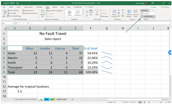
1. Open the Travel Report workbook and select cells A4:E9 in the Jan worksheet.

The first step in creating an outline is to select the cells you wish to summarize.

2. In the Outline group on the Data tab, click the Group drop down arrow and select Auto Outline.

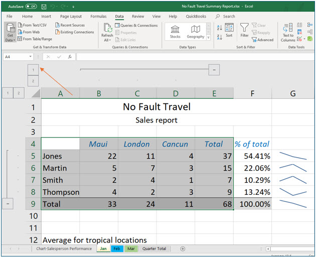
Notice that Excel has added some additional control features above the column headings and to the left of the row headings. Excel has created two outline levels: one vertical level and one horizontal level. As mentioned earlier, more complex worksheets may have more levels.

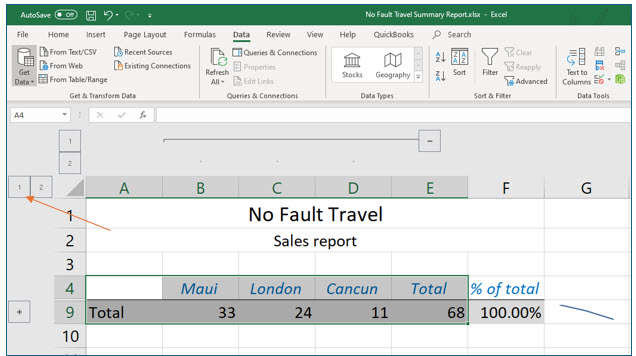
3. Click the level “1” outline button above the column A heading.

This level “1” outline button collapses the column data (destinations) and only the column summaries (all destinations or trips) are shown. We have not changed the outline view of the row data, so we see the trip totals for each salesperson.

4. Expand the column view by clicking the level “2” outline button above the column headings.

We have returned to our original view of all column (destination) data, as well as all row (salesperson) data.

5. Collapse the outline by clicking the level “1” outline button to the left of the row 1 heading.

This level “1” outline button collapses the row data (salespersons) and only the row summaries (all salespersons) are shown. We are looking at totals for each destination.

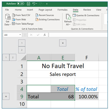
6. Collapse the outline further by clicking the level “1” outline button above the column A heading.

Now, we have also collapsed our column outline view, and we can see only the row and column summary, total trips to all destinations booked by all salespersons.

7. Expand both views by clicking each outline’s “2” level button.

The Auto Outline feature provides an easy way to view and print an “executive summary” of worksheet data. When you no longer have any need for Excel’s outline features, clear the outline, and work in your normal manner.

8. In the Outline group on the Data tab, click the Ungroup tool’s drop-down arrow and choose Clear Outline.

The outlining levels are now removed from this worksheet.

Inserting Cell Notes

Excel allows users to insert notes and comments into cells. For instance, if a value in a worksheet varies greatly from the other values around it, a curious viewer of the spreadsheet may want to know why. This feature is very useful when more than one user is collaborating on a worksheet. After a note is inserted into a cell, any user of that workbook can simply point to that cell and Excel will then display the comment associated with that cell. You can insert comments easily by right-clicking in a cell and choosing Insert Note from the shortcut menu.

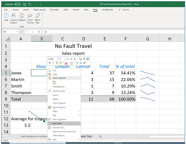
1. Right-click on cell B5 in the Jan worksheet.

Right-clicking brings up a context-sensitive shortcut menu where you can access many common Excel commands and features relevant to what you have selected.

2. Choose New Note from the shortcut menu.

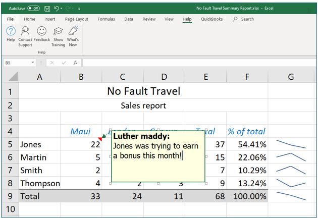
The note text box should now be visible. It displays the name of the user, so that all users of a workbook will know who inserted the note. The name your computer displays (i.e., your identity) will depend on how the computer was installed and your network configuration. You can change the user name as follows: 1) click the File tab; 2) in the Microsoft Office Backstage view, select Options; and 3) on the General Options menu, type desired user name under Personalize your copy of Microsoft Office.

3. After the user name in the comment text box, type Jones was trying to earn a bonus this month! Click anywhere outside the comment box.

You will no longer see the entire note. However, the cell with the note should display a red triangle in the top right corner indicating that this cell has a note. When you point at this cell the comment will expand.

4. Hover over cell B5.

Verify that the note appears when you hover over the cell.

5. Save and Close this workbook.

Protecting Worksheets

After spending valuable time creating a worksheet, you may want to protect it from having someone accidentally erase formulas. Excel allows you to protect cells, so that those cells cannot be changed or erased. Cell protection is very useful when multiple users are collaborating in the same workbook.

When you protect a worksheet, by default, all cells are protected and none can be changed. Typically locked worksheets are not very useful. Normally, you want to allow users to enter certain values used in various computations (contained in locked formulas). To allow users to change the values in specific cells, you must unlock those cells before you protect the worksheet.

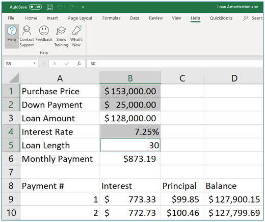
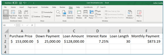
In this portion of this lesson, you will protect the sheet in the Loan Amortization workbook that we created earlier. First you will unlock the cells which require information from the user: the purchase price, down payment, annual interest rate, and number of years for the loan. After you protect the sheet, users will be unable to change any cells that were not unlocked, and this will include all descriptive headers and formulas in the sheet.

1. Open the Loan Amortization workbook.

2. Use the (Control) key to select the non-contiguous cells B1, B2, B4, and B5.

These are the only cells in which users need to provide loan information. Worksheet protection can be turned off, if you ever need to make any changes to the protected portions of the worksheet.

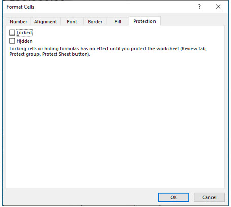
3. Right-click the selected cells to bring up the shortcut menu. Choose Format Cells to launch the Format Cells dialog box.

The Format Cells dialog box will also open using the dialog box launcher in the Font, Alignment, or Number groups on the Home tab.

4. In the Format Cells dialog box, click the Protection tab and turn off the Locked option and click OK.

Cells are locked by default and remain locked until a user unlocks them. You are telling Excel to unlock the selected cells. When you protect a sheet or a workbook, Excel will only protect the locked cells.

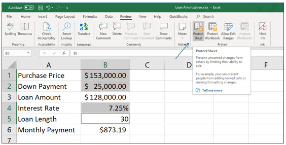
5. In the Protect group on the Review tab, click the Protect Sheet tool.

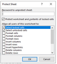
The Protect Sheet dialog box provides options on what users are allowed to do in the protected worksheet. You can also add a password that would be required to unprotect the worksheet. Caution: Use passwords sparingly, especially with company owned data! If you require password protection, make sure someone else in your company also has the password. If you find yourself with a password protected file and you do not have the password, your IT department should be able to help.

6. Click OK to close the Protect Sheet dialog box.

You are not adding a password or changing the actions allowed to users.

In the following step, you will try to alter a protected cell.

7. Move to cell D9 and press (Delete).

A message should appear that this is a protected cell.

8. Click OK in the warning message.

You can only change the contents of cells that were unlocked cells before worksheet protection was turned on.

Using Data Validation and Input Messages

With data validation you can specify the type and range of values which can be entered into unprotected cells. For example, you might require an interest rate between 1% and 10% in the loan amortization worksheet. Setting a validation rule would prevent improper data from being entered into a cell.

When you set validation criteria for a cell (or range of cells), you have the option of creating an instruction, known as an input message, that appears when the cell is selected. An input message might inform the user of the range allowed, such as a range of 1% to 10% for an interest rate. You can also create a custom error message to appear when the user attempts to enter a non-allowed value into the cell.

In this portion of the lesson, you will add data validation to the cell used for entering interest rate in the Loan Amortization worksheet.

1. From the Review tab, in the Protect group, choose Unprotect Sheet.

The sheet is now unprotected, so that you can make changes. After you are finished, you will protect it again. Keep in mind that unless you require password protection, any user can “unprotect” a worksheet or workbook. It is a good idea to keep a master copy of the workbook before distributing it to other users. Moreover, it is always a good idea to have a backup copy of any important file.

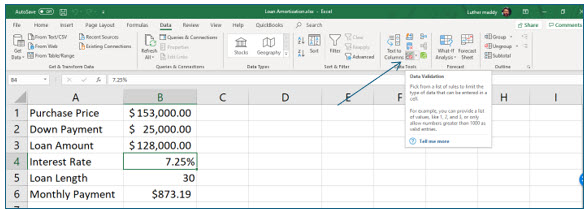
2. Move to cell B4 and select the Data Validation tool in the Data Tools group on the Data tab.

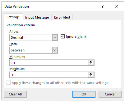
The Data Validation dialog allows you to set the criteria for the values that are allowed in a cell (or range of cells).

3. Under Validation criteria on the Settings tab, select Decimal from the drop-down list under Allow.

You have told Excel to allow decimal values in this cell, instead of whole numbers, dates, or any value at all.

4. Under Validation criteria on the Settings tab, select between from the drop-down list under Data.

You are allowing users to enter a range of values. You could have chosen other operators, such as less than or greater than.

5. Enter 0.01 in the Minimum and 0.1 in the Maximum settings.

Note: Excel does not require that you enter the zero to the left of the decimal point.

The validation criteria ensures that only values in this range will be processed in the loan amortization. Mathematically speaking, 1% is entered in Excel as 0.01, so you are only allowing values between 1% and 10% in this cell.

In the next steps, you will add an input message and a custom error alert to guide workbook users. The input message will provide the acceptable range of values for this cell.

6. Click the Input Message tab in the Data Validation dialog box.

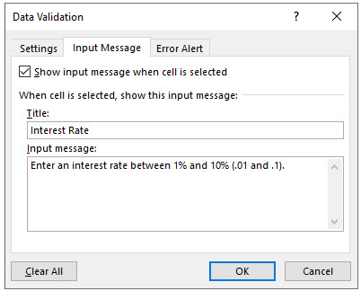
7. Type Interest Rate in the Title and then type Enter an interest rate between 1% and 10% (.01 and .1) in the Input message section.

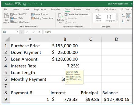
This message will be displayed when users enter cell B4.

Now you will create a custom error message that will appear if the user attempts to enter a value outside the allowable range set by the validation criteria for that cell. If you do not create a custom message, Excel will return a generic error message.

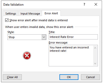
8. Click the Error Alert tab and enter the information shown above in the Title and Error message text areas. When finished, click OK.

The Error Alert text will be displayed if an incorrect interest rate is entered into cell B4.

9. Move to cell B4 and verify that your input message is displayed.

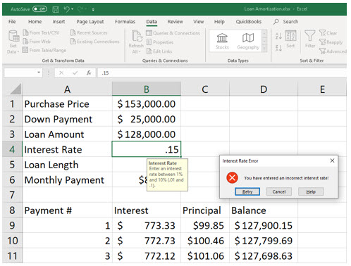
10. In cell B4 type .15 and press (Enter).

The custom error alert should appear to inform you that this value is incorrect.

11. Press (Escape) or click Cancel to return to the original interest rate.

Freezing Worksheet Panes

Large worksheets often cover many pages. When you scroll vertically and horizontally through the worksheet, you may not be able to identify the information you are looking at because the column and row heading are no longer visible.

For example, consider the No Fault Travel Agency and our Travel Report workbook. If the agency added several booking destinations, a total of 20 additional destinations for example, we would we add 20 columns of destination data to our monthly worksheets. As you scroll to the right to enter the number of trips booked to each destination, you may not be able to see each salesperson’s name in the first column. It would be easy to get confused, and mistakenly credit a salesperson who did not book the trip. To prevent this kind of confusion, you can freeze worksheet panes so that column or row headings always remain visible, no matter where you are in the worksheet.

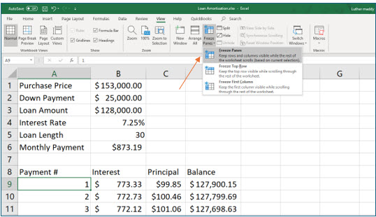
To freeze worksheet panes, move to the row below the rows you want frozen and move to the column to the right of the columns you want frozen. The Freeze Panes tool is located in the Window group on the View tab. In this portion of the lesson you will freeze the panes in the loan amortization schedule

1. Move to cell A9 in Sheet1 of the loan amortization workbook.

You have moved to row 9; when you freeze panes, the first 8 rows will always be visible, even when you scroll down several hundred rows. Since you are located in the first column, column A, you will not freeze any columns because only columns to the left would be frozen.

2. Display the View tab and click the Freeze Panes tool in the Window group.

3. Choose Freeze Panes, the top option from the list of choices.

4. Press (Page Down) several times to scroll down the worksheet.

The loan information and amortization schedule headings in rows 1-8 should be visible.

5. Move back to cell A9 with Control+Home.

When no panes are frozen, Control+Home takes you to cell A1. When panes are frozen, this shortcut takes you to the top of the current pane, in this case, cell A9.

In the next two steps, you will unfreeze the panes and scroll down so you can clearly see the difference that freezing panes makes in a worksheet.

6. Click the Freeze Panes tool again and this time select Unfreeze Panes from the available options.

7. Press (Page Down) several times again.

The loan information and amortization schedule headings in rows 1-8 are no longer visible after you press (Page Down) once.

Using Paste Special: Transpose Data

When you transpose data, you switch the orientation of that data. The original column headings become the new row headings and the original row headings become the new column headings. In this portion of the exercise, you will select and copy the cells that you wish to reorient; then you will move to the location where you want those cells copied and transpose them using the Paste Special options.

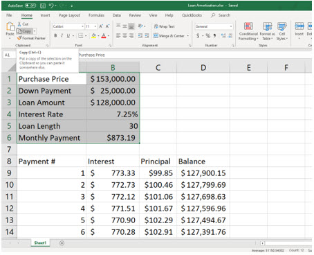
1. In the Loan Amortization workbook, select cells A1 through B6. Click the Copy command in the Clipboard group on the Home tab.

2. Insert a new worksheet. Ensure that cell A1 in the new worksheet is active.

Reminder: To insert a new worksheet, you can simply click the new sheet button (the plus sign inside a circle) next to the tabs for the existing worksheets.

In the next two steps, you will place the copy of the selected cells here.

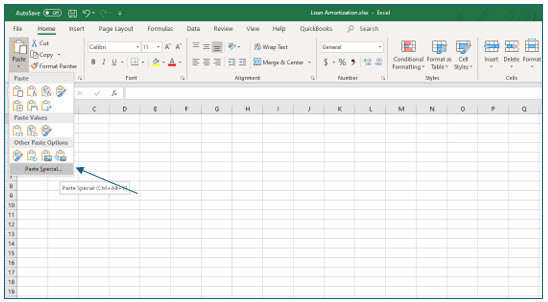
3. On the Home tab, click the drop down arrow on the Paste tool to bring up the Paste menu and then choose Paste Special.

When you hover over a button, a description of the button’s purpose appears. The Transpose button shows the interchange between row and column.

The Paste menu provides you many options for pasting cell contents (Paste group) or pasting cell values only (Paste Values group). The last menu item, Paste Special opens the Paste Special dialog box which lets you select these options, in addition to offering more advanced operations.

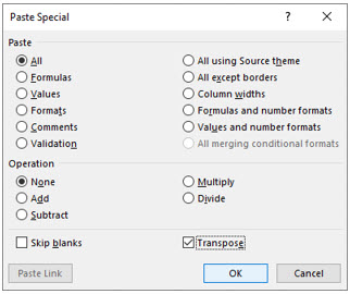
4. In the Paste Special dialog box, turn on the Paste Special check box, and click OK.

You should now see the copied data in a transposed format. Our original cell block spanned six rows and two columns. Our new cell block spans two rows and six columns.

5. Increase the column widths in Sheet2 to accommodate the values contained in the cells.

Hint: Select columns A – F, go to the edge of any selected column and when the pointer transforms into skinny black plus sign with left and right arrows, double-click. Alternatively, use the Format tool in the Cells group on the Home tab.

6. Move back to Sheet1 and protect the worksheet again.

Just in case you need a reminder, you find the Protect sheet tool in the Review tab. All the cells except those you unlocked previously will now be protected. You unprotected the worksheet to add the Data Validation rules and experiment with freezing worksheet panes.