Working with Functions

More Excel Topics
Working with Functions

Working with Functions

This lesson includes step-by-step instructions to teach you to use the PMT(), SumIF(), and VLookup() functions. It will also cover creating and using Named Ranges.

Watch the video-Creating a loan amortization schedule Watch the video-Using Excel's IF funnction Video-Creating an Invoice using the VLookup() fuhnction

Download TripData to complete the lesson

Working with Functions

The functions available in Excel make it easy to perform mathematical operations that would be, at best, very difficult without them. Up to this point you are familiar with at least the Sum and Average functions. Excel has many more very useful functions for just about every computation you may ever want.

Excel’s functions are grouped by category, such and Financial, Statistical, or Math and Trig. Within each category are several useful functions. In this lesson you will get just a small glimpse of some of the power within Excel’s functions.

The PMT() function

The PMT() function allows you to compute loan payments based on a fixed payment amount and fixed interest rate. If you know the amount of the loan, the interest rate and the loan length, Excel’s PMT() function will do the rest. After you have computed a loan payment, it is also then very easy to create a complete loan amortization schedule.

You will now use Excel’s PMT() function to compute a loan payment then create a loan amortization schedule. An amortization schedule displays the breakdown for each payment of the loan, including the amount applied to interest and principal. It also displays the loan balance after each scheduled payment.

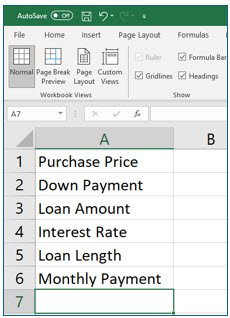
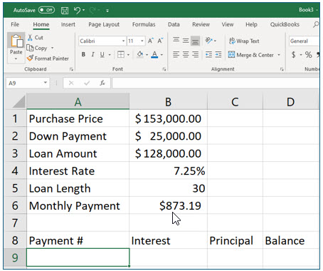
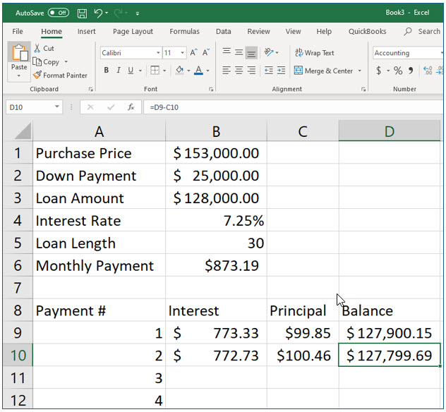
1. In a new workbook, enter the labels as shown below. Change the column width of Column A as needed.

To change column width you can double-click the column’s edge to have Excel adjust the column to the widest value or label in the column. Or, you can click and drag to manually adjust the width.

2. Create a formula in cell B3 that subtracts the Down Payment from the Purchase Price.

The computed value in cell B3 will be the amount that the PMT() function uses to calculate a loan payment. The formula is =B1-B2.

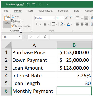
3. Enter the values as shown below. Format the values as shown.

It is not necessary to enter values before creating the formula that computes the loan payment. Placing values in the cells first will make the formula easier to understand as you create it. The loan length is in years, making this a 30-year loan.

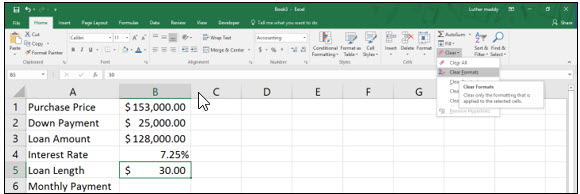
If Excel automatically applies currency formatting to the Loan Length value, you can correct this by using the Clear tool on the Home tab and choosing Clear Formats.

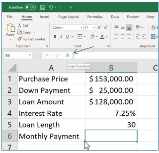
4. Move to cell B6 and then click the Insert Function tool on the Formula bar.

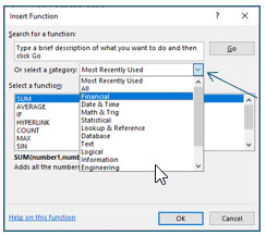
As soon as you click the Insert Function tool, the Insert Function dialog box pops up. By default, Excel displays a list of functions in the “Most Recently Used” category. Excel adds the functions you use to this category, making the functions you commonly use easy to find with the most recent function used being first on the list.

The first time you use a function you may need to locate it manually. If you are not sure how the function is categorized, select the All category. Every function category except the “Most Recently Used” lists the functions alphabetically.

5. Click the Or select a category drop down list and choose the Financial category.

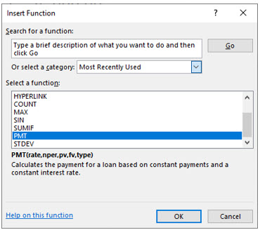
The PMT() function is located in the Financial category.

6. In the Select a function section, select the PMT function and click OK.

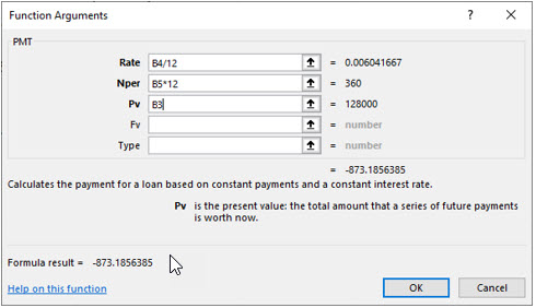
Excel will now display the Function Arguments dialog box which allows you to specify the arguments or parameters you want to use for this function. If the data in the worksheet is hidden by the dialog box, you can easily move the dialog box out of the way by clicking and dragging it to another location on the screen.

7. If needed, move the Function Arguments dialog box so that you can see the values in the worksheet.

8. Enter the arguments for Rate, Nper, and Pv as shown in the Function Arguments dialog box.

Use the (Tab) key, not the (Enter) key, to move from field to field. You can type the cell references or select them with the mouse.

Take the time to read the text in the dialog box. The purpose of the function is explained, as well as the function argument for the active field. Values must be entered into fields for bold-font function arguments. Default values are used if values are not entered in the fields with function argument font is not bold.

You have taken the annual interest rate and divided by 12 to convert it to a monthly interest rate. You have also multiplied the loan length by 12 to provide the total number of monthly payments. When dealing with formulas that depend on time, all time elements should be the same.

9. Click OK to complete the monthly payment formula.

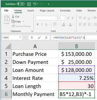
The loan payment amount in cell B6 is displayed in red because Excel has computed a negative number, representing financial outflow (payment). You can create an amortization schedule easier if this number is positive.

10. In cell B6, click in the formula bar and add *-1 at the very end of the formula and press (Enter).

Multiplying a negative value by -1 changes it into a positive value.

In the following steps, you will create a loan amortization schedule. After you have created it, you may use it for your own values if you like.

11. In cell A8 enter Payment #. In cell B8 enter Interest. In cell C8 enter Principal and then enter Balance in cell D8 as shown.

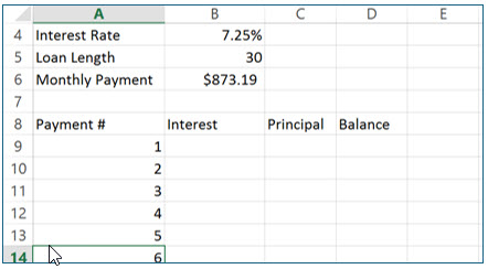
12. Use the fill handle to create incrementing numbers from 1 to 360 in cells A9 through A368.

Type a 1 in cell A9 and a 2 in cell A10. Select both cells; remember, you can select cells when you see the thick white plus sign. Move the mouse pointer to the fill handle, which is the small square in the bottom left corner of your selection. When the thick white plus sign changes to the skinny black plus sign, you have located the fill handle; now click and drag down to cell A368. To replicate a pattern, Excel needs to identify the pattern. Excel interpreted “1,2,…” as a list of numbers with incremental values of one.

The numbers you just placed in column A will become the payments scheduled for this loan, 360 in all because it is a 30 year loan (30 years X 12 months).

You are now ready to create the formulas for the amortization schedule. You will begin by creating the formals for payment #1.

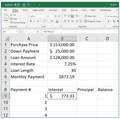
13. In cell B9, create a formula that computes the dollar amount of one month’s interest for the original loan amount: =B3*B4/12

You can manually type the formula or select the reference cells with the mouse. Once again, you are dividing the result by 12 to compute the monthly interest rate.

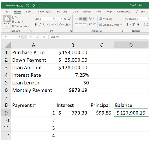
14. In cell C9, create a formula to calculate the amount of the payment which applies to the principal.

This formula is =B6-B9.

15. In cell D9, create a formula which computes the loan balance after making the first payment

This formula is =B3-C9.

The formulas for Payment #1 cannot be copied to the subsequent payments because the relationships are different. In the next three steps, you will create formulas for Payment #2, and use absolute referencing for the interest rate and loan amount, so that the formulas can be copied to do the same calculations for all subsequent payments.

16. In cell B10 enter the formula: =D9*$B$4/12.

This formula refers to the remaining loan balance after making the first payment was made, and uses an absolute (fixed) reference to cell B4, the interest rate.

17. In cell C10, enter the formula =$B$6-B10 to compute the dollar amount of Payment #2 applied to the principal.

This formula subtracts the interest paid from the payment amount, which is a constant value (and does not change).

18. In cell D10, enter the formula =D9-C10 to compute the dollar amount of the remaining loan balance after Payment #2 is made.

The loan balance formula now has a relationship you can copy to the other payments. This formula subtracts the principal amount of this payment from the previous balance.

You are now ready to copy the formulas from payment #2 for the additional payments. To do this you will use the fill handle, but you will also be introduced to a shortcut that can save you even more time when copying formulas with the fill handle.

19. Select cells B10:D10.

You are selecting the formulas for Payment #2. Remember when selecting cells, the mouse pointer should appear as a thick white plus sign rather than the skinny black plus sign, indicating the fill handle.

20. Keeping these cells selected, double-click the fill handle in cell D10.

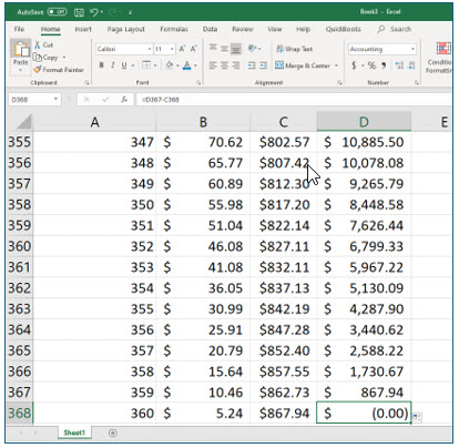
Excel has copied the formulas down through the last payment, Payment #360. When you double-click the fill handle, Excel will copy the contents of the cell until it sees a blank row. This is just one of the great and many reasons that you are learning Excel! You can move to the last cell in this worksheet with Control+End.

21. Save this workbook as Loan Amortization and then close it.

The Vlookup() Function

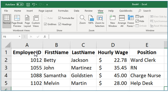
The Vlookup function allows you to look up values located in a table, such as an item’s price based on its part number. Another example would be to look up an employee’s hourly wage based on the employee’s identification number. The values retrieved by the lookup function can be used in formulas, such as calculating costs or wages. This function is very useful for creating invoices or estimates.

An Excel lookup table consists of rows and columns. The first column is the unique value you are looking up, an employee number, in the example table shown above. This value can be a name (text label) or a number, as long as it occurs only once in that column. The values or labels in the first column must be sorted in ascending order for the Vlookup function to work properly. You can use the Vlookup function to return a value contained in any of other columns associated with the looked up value.

In this portion of the exercise, we will create a lookup table which contains No Fault Travel destinations and the cost of the trip per day. We will also create a monthly sales report which tracks the trips booked each month, specifically the following information: trip length and destination, cost, date of the booking, and the salesperson. The VLookup() function is used to return the cost per day associated with a destination.

The syntax for the Vlookup() function is:

=Vlookup(lookup value, lookup table name or cell references, column with the value to be returned)

The Vlookup syntax will make a lot more sense after you use it.

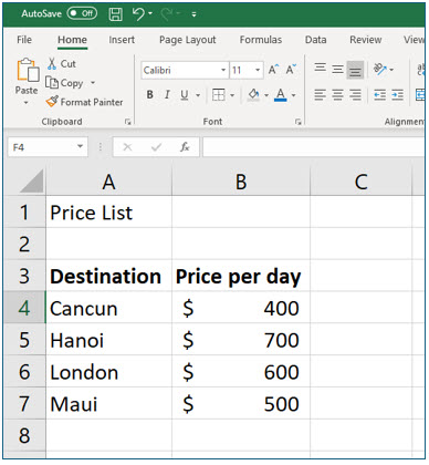
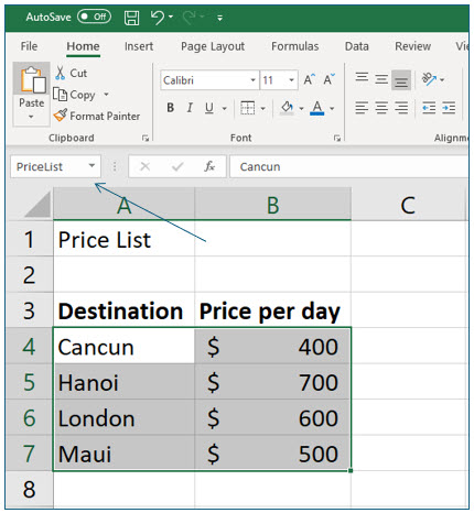
1. Open a new workbook and enter the data shown.

This will become the lookup table you will use in this exercise. You will have Excel find the price per day of a destination when you enter the trip’s destination.

When creating a lookup table, the items in the leftmost column must be sorted numerically or alphabetically in ascending order. This is because the left column in the table is what Excel sees as the key value.

Lookup tables can have several columns of data you want to Excel to find for you, but the left column is the key to finding that information. In the previous example, the EmployeeID was the key value. The example table is a more realistic than what you are using here. We’re keeping it simple for exercise purposes.

(You can always have Excel sort for you, if you do not enter the data with the leftmost column values in ascending order.)

2. Rename Sheet1, Pricing.

Remember, you can double-click the sheet tab to change the sheet’s name.

Creating Named Ranges

Excel allows you to assign names to individual cells or ranges of cells. Naming cells or cell ranges makes it easier to refer to them in formulas, especially when the formulas are copied because named cells and cell ranges are absolutely referenced.

You can name a cell or a range of cells with either of two methods after first selecting the cell or cells you want in the named range. Then you can click on the Formulas tab of the Ribbon and select Define Name from the Defined Names group. Alternatively, you can simply type the name in the Name Box on the left side of the formula bar when the cell or cell range is selected.

1. In Sheet1 (Pricing), Select cells A4:B7. Then, click in the Name Box and type PriceList as the name for this range and press (Enter).

Do not add a space to the range name. Excel does not accept spaces in range names. Notice also that you are not including the column headings in the named range. The headings are there for your benefit, they are not actually part of the lookup table.

You can now refer to cells A4 through A7 on the Pricing worksheet (Pricing!A4:B7) as PriceList in Excel formulas. You will use this name in the lookup formulas you are about to create.

2. Insert a new worksheet and change the sheet name to January.

Names for worksheets and cells are easier to recall and make formulas easier to create.

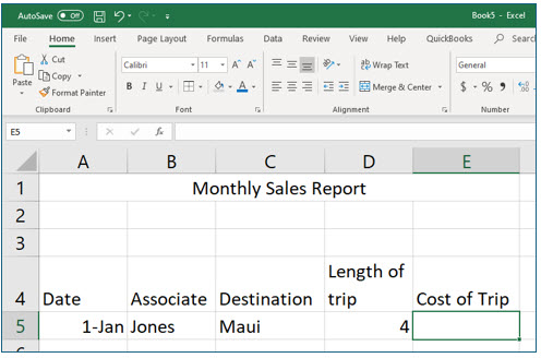
3. In the January worksheet, enter the data shown above.

No matter your skill level in Excel, there will always be more to learn. Although we are working with formulas in this lesson, we have to take a moment to work on our formatting skills. To have the label “Length of trip,” which is too long to fit the width of this column, appear on two lines as shown, you need to turn the Wrap Text option on. You can find this tool on the Home tab in Ribbon, just above the Merge & Center tool.

In the next steps, you will create a formula to calculate the cost of a trip. The formula has two components: 1) use the Vlookup function to return the cost per day for a lookup destination; and 2) multiply the cost per day by the total number of trip days.

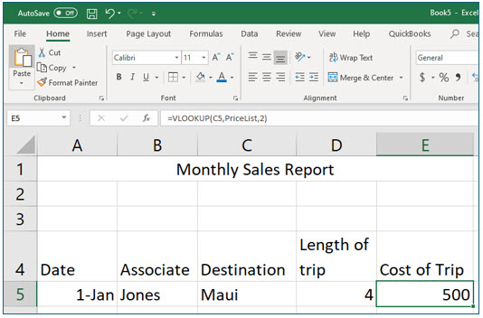
4. Move to cell E5, begin the formula by typing =Vlookup(C5,PriceList,2) and pressing (Enter).

The Vlookup function contains three arguments separated by commas. The first argument, the lookup value, is C5, the destination. The second argument is the lookup table which contains the prices for the destinations. If you have not created a named range, you would refer to the lookup table as: Pricing!A4:B7. The third argument is the column of the lookup table containing the value you would like returned, in this case, destination cost per day.

You should now see that Excel looked up the price per day for Maui. Remember, the goal is to calculate the total cost of the trip, so we need to edit the equation to take the price per day and multiply it by the total number of trip days.

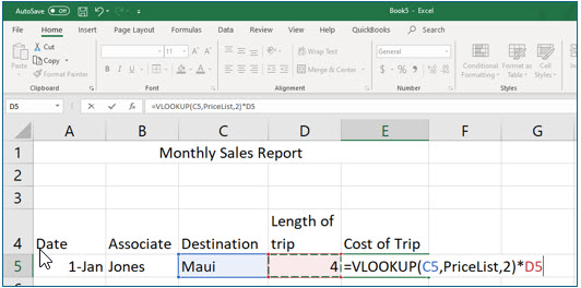
5. Move back into cell E5 and edit the equation, so that the value returned by the Vlookup function is multiplied by cell D5, as shown in the formula bar below.

You now will see the cost of the entire trip based on the value from the Price List table and the trip length.

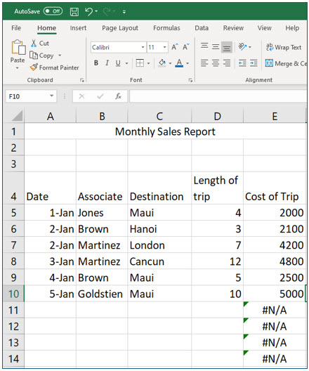
6. Copy the formula in cell E5 through cell E14.

You will see an error message in the empty rows because the cell referenced in the Vlookup function for the lookup value (in our case, the destination) is empty.

7. Enter the additional information as shown. Verify that the total cost for each trip has been computed correctly with our equation using the Vlookup function.

The destinations must be typed exactly as they appear in the price list sheet. If they are spelled differently, or if you added a space after the destination that does not appear in the price list, the formula will not work. If you have problems, ensure everything matches exactly.

8. Save this workbook as Monthly Report by associate but leave it open.

The IF() Function

The If() function is a logical function; it returns one value if the condition is true and another if it is false. We will use the If function to calculate a discount if the total trip cost exceeds a certain amount.

The syntax of the If() function is: =If(Condition to check, value if true, value if false)

The “values” to be returned can be computations. In the next steps, you will use the If() function to compute a customer’s discount based on the cost of the trip.

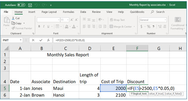
1. In the Monthly Report by associate workbook, move to cell F4 in the January worksheet, type Discount and then press (Enter).

The No Fault Travel agency gives a 5% discount, if the total cost of the trip exceeds $2,500. Let’s frame the If() statement in our minds.

Arguments for IF() Mathematical expression Logical test: Does trip exceed $2,500? Trip cost > 2500 Discount if True Trip cost x 0.05 Discount if False 0

2. In cell F5 type the following formula: =IF(E5>2500,E5*0.05,0)

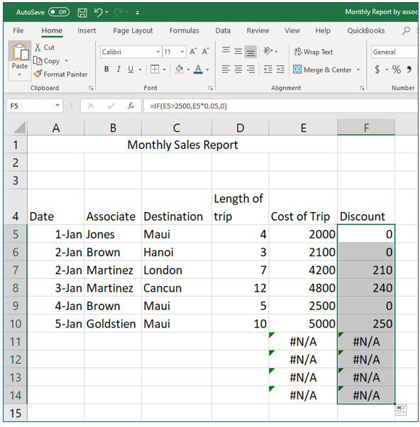
3. Copy the formula from F5 through F14.

You may double-click the fill handle on cell F5 to quickly copy this discount formula. Add accounting formatting as shown.

Nested If Statements

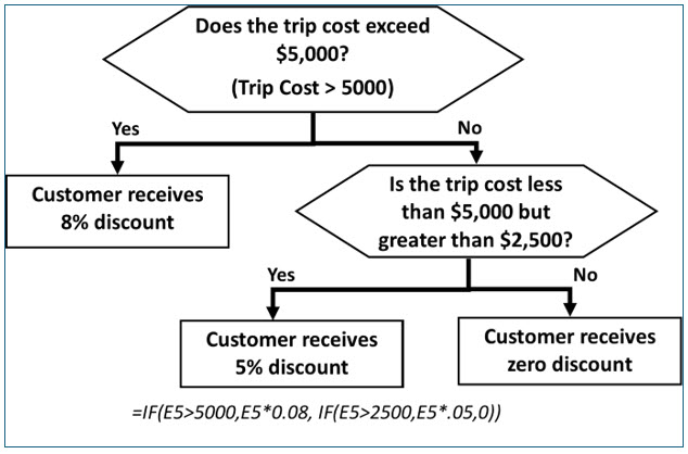
Multiple If() functions (up to 64) can be used in the same formula to return different values in situations where there are more than two possible outcomes. For example, if you wanted higher trip costs to qualify for a higher percentage discount, the following formula could be used: =IF(E5>5000,E5*0.08, IF(E5>2500,E5*.05,0))

Let’s try to evaluate our equation for this situation of three possible outcomes.

Conditional Summing: SumIf()

In addition to the stand-alone If() function, the Excel function libraries contain additional conditional functions, including a few statistical functions, such as SumIf(), AverageIf(), and CountIf(). These functions execute their normal functions if the conditional statement is true. For example, if you wanted to know the total cost of all the trips to Maui, you could use the SumIf() function to sum the trips to Maui.

In the next portion of the lesson, you will create a formula that adds only the trip costs to specific destinations.

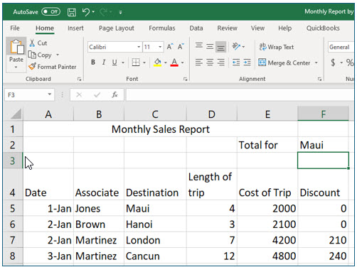
1. Move to cell E2 and type Total for, and then press the right arrow key () to move to cell F2.

2. In cell F2 type Maui and then press the right arrow key ().

The destination, in this case Maui, should be placed in a separate cell because it is the criteria we are using in the SumIf function to determine if the trip cost should be included in the total.

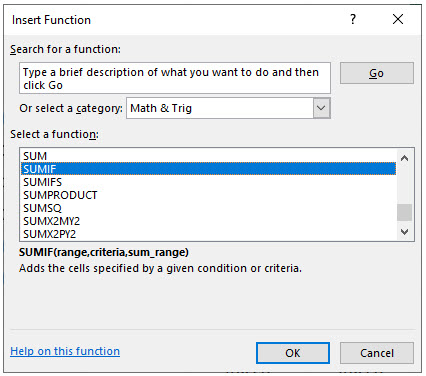
3. Move to cell G2 and begin a formula by clicking the Insert Function tool at the left edge of the formula bar.

4. Locate the SUMIF function and click OK.

You can find this function in Math & Trig, but if you are not sure which library contains function, all functions are included in the All category.

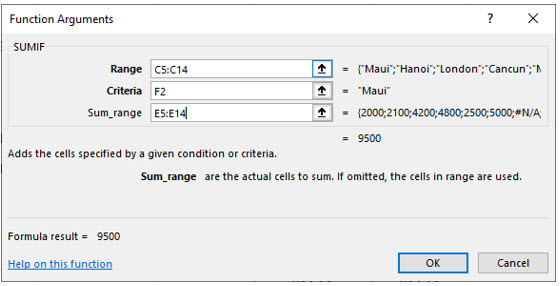
You should now see the Function Arguments dialog box which will help you build this formula.

5. In the Range text box type or select C5:C14.

This is the evaluation range. The cells in this range are evaluated to see if they meet the criteria. In this case, the evaluation range is the destination of the booked trips, and the criteria is the destination you specify (i.e., Maui).

6. In the Criteria text box type or click on cell F2.

The criteria is the cell where you will type the destination you want to total the trips for.

7. In the Sum Range type or select cells E5:E14.

The sum range contains the values which will be included in the sum if the condition or criteria is met.

8. Click OK after entering the correct parameters.

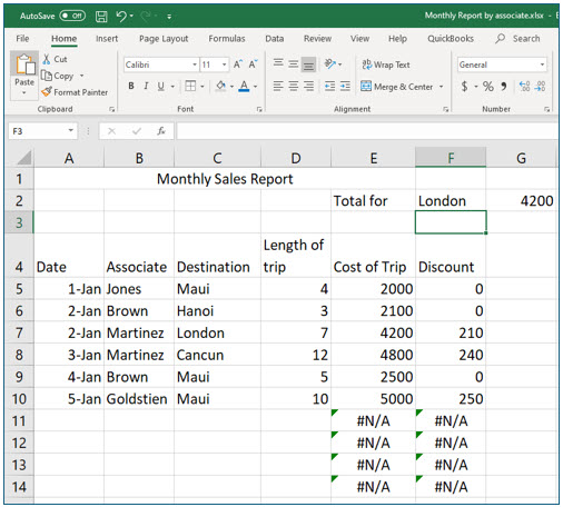
You should now see the total cost of all the trips to Maui in cell G2. Verify that the total cost is correct.

9. Change the destination in cell F2 to London.

Cell F2 provides the criteria for the conditional function. Verify that the sum of the cost of the trips to London is correct.