Using Functions and Absolute Reference

More Excel Topics
Using Functions and Absolute Reference

Using Functions and Absolute Reference

The step-by-step instructions in this lesson explain how to use the Sum and Average Function. It also explains how and why to use Absolute Cell Referencing in formulas in Excel

Watch the video-Creating basic formulas and using functions

Watch - How & Why to use Absolute Reference

Download Excel Functions Exercise File

Using Functions and Absolute Reference

Excel provides several shortcuts when you are creating what could be fairly complex formulas. So far, you have already used one Excel function, the Sum function. As you should recall, the Sum function made it possible to add several cells in a very simple formula.

In addition to the Sum function, Excel has numerous other functions. In this lesson you will explore some of Excel’s basic functions. After you’ve done that, you’ll then learn more about copying formulas and you’ll learn the important feature called Absolute Reference.

The Go to Command

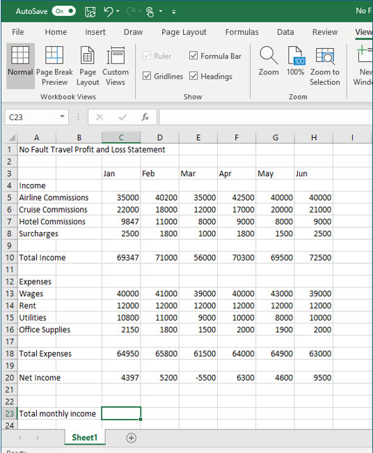
1. Open the No Fault Travel P&L workbook.

You can use the mouse to quickly click and go to any cell you see. However, if you wish to quickly move to a cell you cannot see, even one that is quite far away, you can use the Go to command.

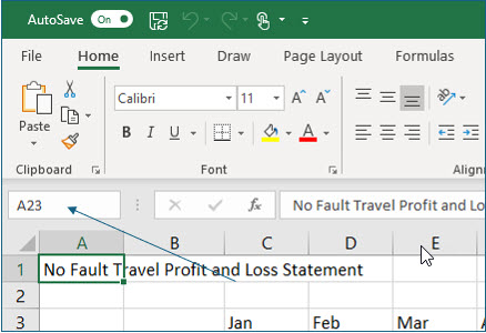
The easiest way to access the Go to command is from the name box. To move to another cell, just type that cell’s address in the name box and press (Enter). Excel will then instantly move you to that cell. You can also access the Go to command with the F5 function key.

2. Click in the Name box, type A23 and then press (Enter).

Be sure that you don’t put a space between the A and the 23.

As you pressed (Enter), Excel moved the active cell to A23.

3. In cell A23 type, Total Monthly Income and press the (Right) arrow twice to move to cell C23.

When you used the Sum function earlier, you used the AutoSum tool. This tool simply adds all the values it sees above or to the left of the current cell. In this case, you will use the Sum function but manually inform Excel which cells to add.

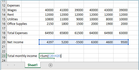
4. In cell C23 type =Sum(C20:H20) and press (Enter).

The parentheses () are a necessary component when using functions of any kind.

This formula will add all the monthly incomes together.

Using additional functions

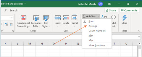
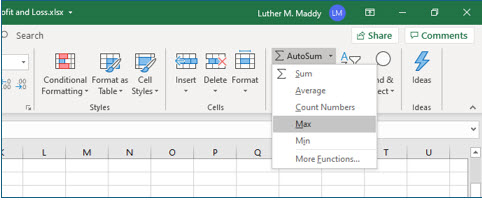
There are many additional functions available for you to use in Excel. In this portion of the lesson you will use the Average, Max, and Min functions. These functions are readily available from the drop down list button on the AutoSum tool.

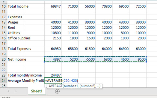
1. Move to cell A24 and type Average Monthly Profit and press (Right) twice to move to cell C24.

You may not be able to see all of the text you just typed. Don’t worry about this, you will learn to increase column widths in the next lesson.

2. Locate and click the arrow just to the right of the AutoSum tool on the toolbar. Then, click Average from the drop down list.

Excel will now place the Average function in cell C24. Excel tries to guess which cells you want to average, which in this case is not correct. The next step is to tell Excel which cells you want to average which, for this worksheet, are cells C20 : H20. You can now either type those cells into the formula within the parenthesis or click and drag to select the cells. For example purposes, you’ll select the cells to be averaged by clicking and dragging.

3. Select cells C20 through H20 by clicking and dragging.

Be sure to select cells using the “fat white plus” in the middle of the cell.

When you release the mouse you will see a marquee around those cells. You will also see C20:H20 has been added to the Average function in cell C24.

4. Press (Enter) to complete the formula.

You should now see the average net income in cell C24. The formula bar will display the formula based on the Average function.

5. Move to cell A25 and type Highest Monthly Profit and then move to cell C25.

You will now use the Max function to display the largest monthly profit value.

6. Click the arrow just to the right of the AutoSum tool on the toolbar and choose Max from the drop down list.

7. Select cells C20 through H20 by clicking and dragging and then press (Enter).

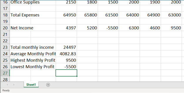
8. In cell A26 type, Lowest Monthly Profit. Then, using the drop down list by the AutoSum tool, insert the Min function. Select cells C20 through H20 and press (Enter).

You should now have formulas that compute the total, average, maximum, and minimum monthly profit values.

Even though the contents of these cells appear to extend into column B, the entire contents are actually in column A. These are examples of “long labels”.

9. Move to cell A21 and type % of Total Income and then press (Right) twice.

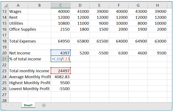
You will now create a formula that computes the percentage January contributed to the total profit for the six-month period. Eventually you will compute the percentages for each of the six months.

10. In cell C21 enter the following formula: =C20/C23.

This formula divides January’s profit by the total profit for all six months.

11. Press (Enter) to complete this formula.

Excel should display a value close to 0.179. This value is actually 17.9%. You’ll add the percentage formatting in a future lesson.

12. Use the Fill handle and copy this formula into cells D21 through H21.

Remember the Fill handle is the “skinny black plus”.

Using Absolute Reference

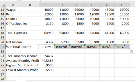
The result of copying the formula into cells D21 through H21 is an error message. You have received this error message because this formula is not a formula that can be correctly copied. You may recall that when you copy a formula, you copy what the formula does in relation to the cell where you copy it to.

In other words, the formula in C21 is C20/C23. Excel actually sees this as: divide the cell immediately above this cell (C20) by the cell two below this cell (C23). If you examine the formula in cell D21 you will see that it became D20/D23 when you copied it. Excel replicated the exact relationship the formula represented and adjusted the cells to the new cell. This is what formulas are supposed to do when you copy them, but this is not the result you are after.

Examining the formulas in E21 through H21 will reveal that each formula refers to two cells in the same column in which the formula is located. The actual error message is telling you that you are trying to divide by zero, a mathematical “no no”. There is no data in cells D23 through H23.

In this situation, you don’t want every part of the formula to change. Instead you’ll need every formula to always refer to the one cell that contains the Total Monthly Profit, cell C23. There are two solutions to this problem. One is to manually change each formula to refer to cell C23. The second, and preferred solution, is to change the way Excel treats C23 when it copies the formula.

Since you want all the other formulas to refer to C23 when you copy the formula to the other cells, you need to tell Excel to keep it constant, or absolute, when the formula is copied. You will not change the way Excel treats C21 because you do want this to change to D21 and so on.

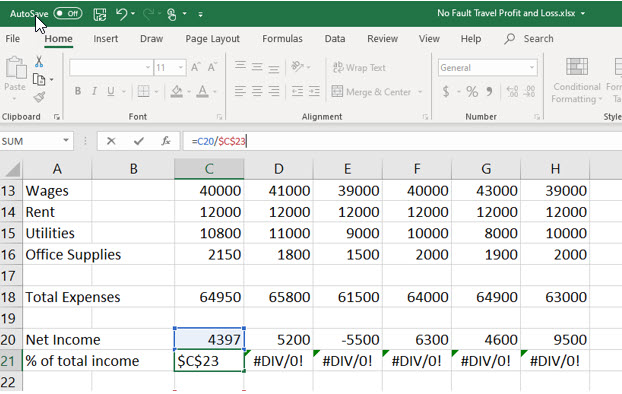
The feature to do this is called absolute reference. In a formula, absolute reference is indicated with ($). For example C21/$C$23 would keep C23 as a constant when you copy that formula.

You can change a cell to an absolutely referenced cell either by typing the dollar signs in manually or by using (F4). In this portion of the lesson you will use absolute reference to make the formula in cell C21 one that can be copied.

1. Move back into cell C21 and click at the far right end of its formula on the formula bar.

2. With the insertion point blinking at the end of the formula, press (F4).

The F4 key adds dollar signs ($) before the row and the column. This key is a shortcut key for making a cell absolute. You can also simply add the dollar signs yourself by editing the formula. The dollar sign before the row and column tell Excel not to change this portion of the formula at all when you copy it.

There are variations of the absolute reference. For example, $C23 would tell Excel to keep column C constant but change the row when you copy to a new location. Likewise, C$23 would keep the row constant. For this formula, you want all the other places you copy it to refer to the total of all the monthly incomes in cell C23. To do this requires a dollar sign ($) before the column and the row.

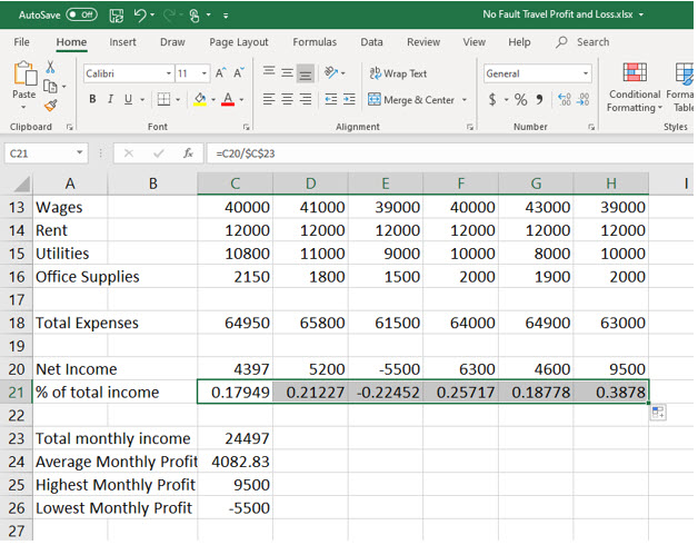
Making cell C23 absolute in the formulas in cells D21 through H21 will cause Excel to display the correct percentage. You can now correctly copy the revised formula.

3. Use the fill handle to copy the corrected formula from C21 to D21 through H21.

This time you are able to copy the formula with correct results because you used absolute reference. You will add percentage formatting, (%), in an upcoming lesson.

4. Examine the formulas in cell D21 through H21.

Notice that each of these formulas now refers to cell C23. C23 did not change this time when you copied the formula because it was absolutely referenced.