Creating a Loan Amortization Schedule in Excel
Note: These instructions are an excerpt of Luther Maddy’s Excel Beyond the Basics. This full text is available in printed or eBook format from Amazon.com
The PMT() function allows you to compute loan payments based on a fixed payment amount and fixed interest rate. If you know the amount of the loan, the interest rate and the loan length, Excel’s PMT() function will do the rest. After you have computed a loan payment, it is also then very easy to create a complete loan amortization schedule.
Here's some step-by-step instructions to compute a loan payment then create a loan amortization schedule. An amortization schedule displays the breakdown for each payment of the loan, including the amount applied to interest and principal. It also displays the loan balance after each scheduled payment.
Watch the video-Creating a loan amortization schedule
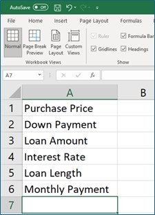
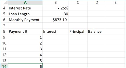
1. In a new workbook, enter the labels as shown below. Change the column width of Column A as needed.
To change column width you can double-click the column’s edge to have Excel adjust the column to the widest value or label in the column. Or, you can click and drag to manually adjust the width.
Printable Instructions - Creating a loan amortization schedule
Download completed Loan Amortization Schedule template
2. Create a formula in cell B3 that subtracts the Down Payment from the Purchase Price.
The computed value in cell B3 will be the amount that the PMT() function uses to calculate a loan payment. The formula is =B1-B2.
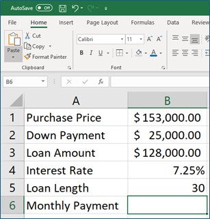
3. Enter the values as shown below. Format the values as shown.
It is not necessary to enter values before creating the formula that computes the loan payment. Placing values in the cells first will make the formula easier to understand as you create it. The loan length is in years, making this a 30-year loan.
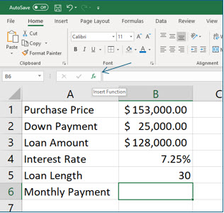
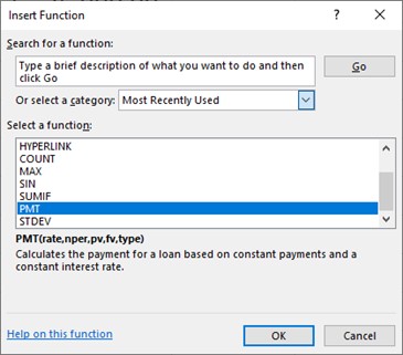
4. Move to cell B6 and then click the Insert Function tool on the Formula bar.
As soon as you click the Insert Function tool, the Insert Function dialog box pops up. By default, Excel displays a list of functions in the “Most Recently Used” category. Excel adds the functions you use to this category, making the functions you commonly use easy to find with the most recent function used being first on the list.
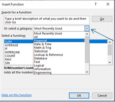
5. Click the Or select a category drop down list and choose the Financial category.
6. In the Select a function section, select the PMT function and click OK.
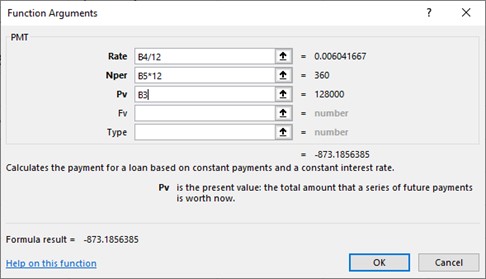
Excel will now display the Function Arguments dialog box which allows you to specify the arguments or parameters you want to use for this function. If the data in the worksheet is hidden by the dialog box, you can easily move the dialog box out of the way by clicking and dragging it to another location on the screen.
7. If needed, move the Function Arguments dialog box so that you can see the values in the worksheet.
8. Enter the arguments for Rate, Nper, and Pv as shown in the Function Arguments dialog box.
Use the (Tab) key, not the (Enter) key, to move from field to field. You can type the cell references or select them with the mouse.
Take the time to read the text in the dialog box. The purpose of the function is explained, as well as the function argument for the active field. Values must be entered into fields for bold-font function arguments. Default values are used if values are not entered in the fields with function argument font is not bold.
You have taken the annual interest rate and divided by 12 to convert it to a monthly interest rate. You have also multiplied the loan length by 12 to provide the total number of monthly payments. When dealing with formulas that depend on time, all time elements should be the same.
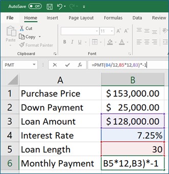
9. Click OK to complete the monthly payment formula.
The loan payment amount in cell B6 is displayed in red because Excel has computed a negative number, representing financial outflow (payment). You can create an amortization schedule easier if this number is positive.
10. In cell B6, click in the formula bar and add *-1 at the very end of the formula and press (Enter).
Multiplying a negative value by -1 changes it into a positive value.
In the following steps, you will create a loan amortization schedule. After you have created it, you may use it for your own values if you like.
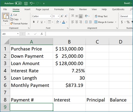
11. In cell A8 enter Payment #. In cell B8 enter Interest. In cell C8 enter Principal and then enter Balance in cell D8 as shown.
12. Use the fill handle to create incrementing numbers from 1 to 360 in cells A9 through A368.
Type a 1 in cell A9 and a 2 in cell A10. Select both cells; remember, you can select cells when you see the thick white plus sign. Move the mouse pointer to the fill handle, which is the small square in the bottom left corner of your selection. When the thick white plus sign changes to the skinny black plus sign, you have located the fill handle; now click and drag down to cell A368. To replicate a pattern, Excel needs to identify the pattern. Excel interpreted “1,2,…” as a list of numbers with incremental values of one.
To replicate a pattern, Excel needs to identify the pattern. Excel interpreted “1,2,…” as a list of numbers with incremental values of one.
The numbers you just placed in column A will become the payments scheduled for this loan, 360 in all because it is a 30 year loan (30 years X 12 months).
You are now ready to create the formulas for the amortization schedule. You will begin by creating the formals for payment #1.
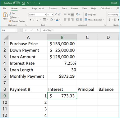
13. In cell B9, create a formula that computes the dollar amount of one month’s interest for the original loan amount: =B3*B4/12
You can manually type the formula or select the reference cells with the mouse. Once again, you are dividing the result by 12 to compute the monthly interest rate.
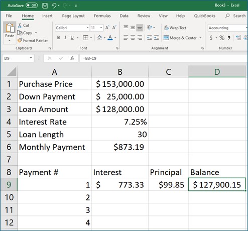
14. In cell C9, create a formula to calculate the amount of the payment which applies to the principal.
This formula is =B6-B9.
15. In cell D9, create a formula which computes the loan balance after making the first payment.
This formula is =B3-C9.
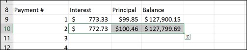
The formulas for Payment #1 cannot be copied to the subsequent payments because the relationships are different. In the next three steps, you will create formulas for Payment #2, and use absolute referencing for the interest rate and loan amount, so that the formulas can be copied to do the same calculations for all subsequent payments.
16. In cell B10 enter the formula: =D9*$B$4/12.
This formula refers to the remaining loan balance after making the first payment was made, and uses an absolute (fixed) reference to cell B4, the interest rate.
17. In cell C10, enter the formula =$B$6-B10 to compute the dollar amount of Payment #2 applied to the principal.
This formula subtracts the interest paid from the payment amount, which is a constant value (and does not change).
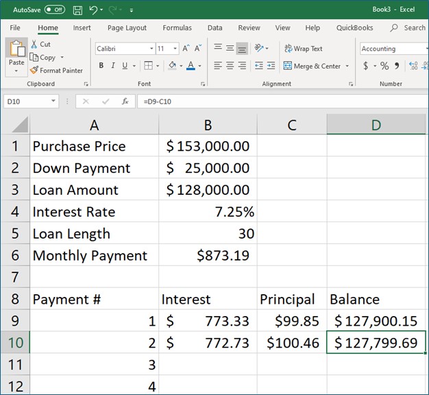
18. In cell D10, enter the formula =D9-C10 to compute the dollar amount of the remaining loan balance after Payment #2 is made.
The loan balance formula now has a relationship you can copy to the other payments. This formula subtracts the principal amount of this payment from the previous balance.
You are now ready to copy the formulas from payment #2 for the additional payments. To do this you will use the fill handle, but you will also be introduced to a shortcut that can save you even more time when copying formulas with the fill handle.
19. Select cells B10:D10.
You are selecting the formulas for Payment #2. Remember when selecting cells, the mouse pointer should appear as a thick white plus sign rather than the skinny black plus sign, indicating the fill handle.
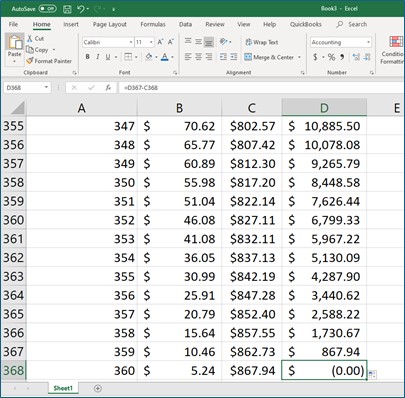
20. Keeping these cells selected, double-click the fill handle in cell D10.
Excel has copied the formulas down through the last payment, Payment #360. When you double-click the fill handle, Excel will copy the contents of the cell until it sees a blank row. This is just one of the great and many reasons that you are learning Excel! You can move to the last cell in this worksheet with Control+End.
21. Save this workbook as Loan Amortization and then close it, and then use it anytime you need a loan amortization schedule.